This article was published as a part of the Data Science Blogathon.
Introduction on Binary Classification
Artificial Intelligence, Machine Learning and Deep Learning are transforming various domains and industries. One such domain is the field of Healthcare. ML is used in healthcare for a variety of purposes. It allows healthcare providers to generate massive amounts of data and make critical clinical decisions. By analyzing thousands of healthcare records and other patient data, ML algorithms can detect patterns associated with diseases and health conditions. They can also aid in the detection of tumours on scans and the identification of potential health issues. Wearable devices and sensors that monitor things like steps, oxygen levels, and heart rates generate a large amount of data that allows doctors to assess the health of their patients in real-time.
Skin cancer is the most prevalent type of cancer, accounting for at least 40% of all cancer cases worldwide. It is one of the leading causes of death in the world. In this article, we will try to perform binary classification using deep learning on the Skin Cancer: Malignant vs. Benign dataset, which is available on Kaggle. You can either download the dataset from here or create a new notebook and run it on Kaggle.
Overview of the Dataset
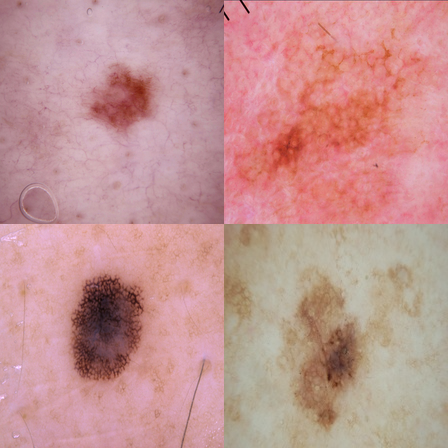
The dataset contains 3600 images of benign skin moles and malignant skin moles. The dataset is balanced. The dataset has 2 major folders namely test and train. Both the train and test folder contain 2 folders namely benign and malignant. Inside the train folder, the benign folder has 1440 images while the malignant folder has 1197 images. Inside the test folder, the benign folder has 360 images while the malignant folder has 300 images. All the images have the same dimension – 224×244.
These are few images from the dataset that we will be using in this article.

Importing Modules
For loading and processing images, we will be using OpenCV and for building and training the neural network, we will be using TensorFlow and Keras. We will be using the Xception model with image-net dataset weights for the neural network architecture and building on top of it. This is not the same as transfer learning. In transfer learning, we freeze layer weights to reduce computation time and complexity, so the weights don’t get updated. Here, I will not freeze the layer weights.
import numpy as np
import os
from sklearn.preprocessing import LabelEncoder
import cv2
from tensorflow.keras.layers import Dense, Conv2D, Flatten, Dropout, MaxPooling2D
from tensorflow.keras.optimizers import Adam
from tensorflow.keras.models import Sequential
from sklearn.model_selection import train_test_split
from tensorflow.keras.callbacks import ReduceLROnPlateau,EarlyStopping
from tensorflow.keras.applications import Xception
Dataset Loading and Preprocessing
Now that we have imported all the necessary modules, let us load the training dataset. As mentioned earlier, each image is a square image with 224*224 pixels. OpenCV uses the BGR format and not the conventional RBG format. So, we will first convert it to the traditional RBG format, resize each image into 200×200 pixels and normalize the pixel values to simplify the computation. Along with loading the data, we will also create the respective target column for training and evaluating our neural network.
ben = os.listdir('../input/skin-cancer-malignant-vs-benign/train/benign')
mal = os.listdir('../input/skin-cancer-malignant-vs-benign/train/malignant')
# Let benign be 0 and malignant be 1
train = []
train_y = []
for i in ben:
    x = '../input/skin-cancer-malignant-vs-benign/train/benign/' + i
    img = cv2.cvtColor(cv2.imread(x), cv2.COLOR_BGR2RGB)
    img = cv2.resize(img,(200,200))
    img = img/255 # normalising
    train.append(img.flatten())
    train_y.append(0)
for i in mal:
    x = '../input/skin-cancer-malignant-vs-benign/train/malignant/' + i
    img = cv2.imread(x)
    img = cv2.cvtColor(img, cv2.COLOR_BGR2RGB)
    img = cv2.resize(img,(200,200))
    img = img/255 # normalising
    train.append(img.flatten())
    train_y.append(1)
train = np.array(train)
Train and Validation Split
We will split our processed dataset into train data and validation data using the 80-20 rule. Validation data is not the same as test data. The validation dataset is unseen by the neural network and is used to evaluate the model on every epoch. The test dataset is the unseen dataset that is used to evaluate the trained neural network.
train,val,train_y,val_y = train_test_split(train,train_y,test_size=0.2,random_state=44)
train = train.reshape(train.shape[0],200,200,3)
val = val.reshape(val.shape[0],200,200,3)
encoder = LabelEncoder()
encoder = encoder.fit(train_y)
train_y = encoder.transform(train_y)
encoder = encoder.fit(val_y)
val_y = encoder.transform(val_y)
print(str('training rows ' + str(len(train))))
print(str('validation rows ' + str(len(val))))
We can see that there are 2109 samples in the training dataset and 528 samples in the validation dataset.
training rows 2109
validation rows 528
Building the Neural Network
Since we have an image dataset in hand, CNN is the best option out there. Every CNN model has 2 parts namely the convolution part and the neural network part. The convolution part performs a convolution operation on the input image and extracts low level and high-level features from it. These extracted features are then used to model a neural network to classify the input. As mentioned earlier, we will be using the Xception model with the image-net weights for the convolution part alone. We will make all the layers in the Xception model trainable instead of freezing them and performing transfer learning. We will manually create the neural network part. The input will be an image (which is basically a matrix) having dimension (200x200x3) while the output will be an integer – 0 for benign and 1 for malignant. Dropout layers are simple yet effective in handling the problem of overfitting. A dropout layer randomly selects a portion of neurons and turns them off during the training phase which makes the model more generalized and prevents overfitting. Dropout layers function only during the training phase and not while evaluating. The output layer has one neuron, as it is a binary classification, with a sigmoid function as the activation function. We will be using Adam as the optimizer and binary cross-entropy as the loss function for training the model.
model = Sequential()
base = Xception(include_top=False, weights="imagenet", input_shape=(200,200,3), pooling='avg')
for lay in base.layers: lay.trainable = True # false for transfer learning
model.add(base)
model.add(Dropout(0.8))
model.add(Flatten())
model.add(Dense(64,'relu'))
model.add(Dropout(0.6))
model.add(Dense(1,'sigmoid'))
model.compile(Adam(0.0001),'binary_crossentropy',['accuracy'])
model.summary()
This is the model’s architecture.
Model: "sequential"
_________________________________________________________________
Layer (type)                 Output Shape              Param #
=================================================================
xception (Functional)        (None, 2048)              20861480
_________________________________________________________________
dropout (Dropout)            (None, 2048)              0
_________________________________________________________________
flatten (Flatten)            (None, 2048)              0
_________________________________________________________________
dense (Dense)                (None, 64)                131136
_________________________________________________________________
dropout_1 (Dropout)          (None, 64)                0
_________________________________________________________________
dense_1 (Dense)              (None, 1)                 65
=================================================================
Total params: 20,992,681
Trainable params: 20,938,153
Non-trainable params: 54,528
_________________________________________________________________
Keras Callbacks
We will be using a couple of callbacks while training our model. We will use early stopping to prevent overfitting of the model and this basically stops the training process based on the condition specified by us. For example, say we want to stop the training if the validation loss does not decrease over 5 epochs, in such a scenario early stopping comes into the picture. It can monitor any parameter like training accuracy, validation accuracy, training loss and validation loss for a specified number of epochs. Along with early stopping, we will also use reduce learning rate on a plateau which basically reduces the learning rate by a factor specified by the user. You can read more about the callbacks offered by Keras here.
reduce_lr = ReduceLROnPlateau(monitor='val_loss', patience=2, verbose=2, factor=0.3, min_lr=0.000001)
early_stop = EarlyStopping(patience=4,restore_best_weights=True)
Training
We can now train the CNN on the training dataset and validate it on the validation dataset after each epoch.
model.fit(train,train_y,epochs=25,batch_size=10,validation_data=(val,val_y),verbose=2,callbacks=[early_stop,reduce_lr])
Evaluating
Now, it is time to evaluate our trained CNN on the unseen test dataset. We need to preprocess the test data as we did on our training set before feeding it to the trained model for evaluation.
ben = os.listdir('../input/skin-cancer-malignant-vs-benign/test/benign')
mal = os.listdir('../input/skin-cancer-malignant-vs-benign/test/malignant')
test = []
test_y = []
for i in ben:
    x = '../input/skin-cancer-malignant-vs-benign/test/benign/' + i
    img = cv2.imread(x)
    img = cv2.cvtColor(img, cv2.COLOR_BGR2RGB)
    img = cv2.resize(img,(200,200))
    img = img/255 # normalising
    test.append(img)
    test_y.append(0)
for i in mal:
    x = '../input/skin-cancer-malignant-vs-benign/test/malignant/' + i
    img = cv2.imread(x)
    img = cv2.cvtColor(img, cv2.COLOR_BGR2RGB)
    img = cv2.resize(img,(200,200))
    img = img/255 # normalising
    test.append(img)
    test_y.append(1)
test = np.array(test)
encoder = LabelEncoder()
encoder = encoder.fit(test_y)
test_y = encoder.transform(test_y)
loss,acc = model.evaluate(test, test_y,verbose=2)
print('Accuracy on test data: '+ str(acc*100))
print('Loss on test data: ' + str(loss))
We achieved an accuracy of 87.8% with a loss of 0.3 on the test dataset.
21/21 - 2s - loss: 0.3007 - accuracy: 0.8788
Accuracy on test data: 87.87878751754761
Loss on test data: 0.3006673753261566
Conclusion on Binary Classification
In this article, we built a CNN based binary classification on a pre-trained model (Xception) with image-net dataset weights, made the Xception model’s layers trainable, and used the skin cancer dataset to train the CNN and distinguish benign and malignant moles from images with an accuracy of 87.8%.
We can further continue this project by performing transfer learning using different pre-trained models. In the case of transfer learning, we need to set the trainable property of each layer of the pre-trained model to false. This will stop the weights of the pre-trained model from being updated and makes the training process faster. We can also perform image augmentation and make the model more generalized.
There are multiple medical datasets available on Kaggle. They could be used to build machine learning and deep learning models for learning and also aid in the detection of diseases. Medical datasets are special. Most of them have the problem of class imbalance. Handling the class imbalance problem becomes a necessity on such datasets. Medical datasets are great for learning new things. I will try to cover the class imbalance handling techniques in the coming weeks. Alternatively, you could explore various class imbalance handling techniques and use them on different datasets and comment on how they helped in improving your machine learning and deep learning models.
You can download the code to run this whole project on a Kaggle notebook from here.
Thanks for reading and happy learning!
The media shown in this article is not owned by Analytics Vidhya and is used at the Author’s discretion.


