Beginners Guide to Artificial Neural Network

This article was published as a part of the Data Science Blogathon

Introduction

Deep Learning which is a subset of Machine Learning is the human brain embedded in a machine. It is inspired by the working of a human brain and therefore is a set of neural network algorithms which tries to mimics the working of a human brain and learn from the experiences.

In this article, we are going to learn about how a basic Neural Network works and how it improves itself to make the best predictions.

Table of Content

1. Neural networks and their components
2. Perceptron and Multilayer Perceptron
3. Step by Step Working of Neural Network
4. Back Propagation and how it works
5. Brief about Activation Functions

Artificial Neural Networks and Its components

Neural Networks is a computational learning system that uses a network of functions to understand and translate a data input of one form into a desired output, usually in another form. The concept of the artificial neural network was inspired by human biology and the way neurons of the human brain function together to understand inputs from human senses.

In simple words, Neural Networks are a set of algorithms that tries to recognize the patterns, relationships, and information from the data through the process which is inspired by and works like the human brain/biology.

Components / Architecture of Neural Network

A simple neural network consists of three components :

• Input layer
• Hidden layer
• Output layer

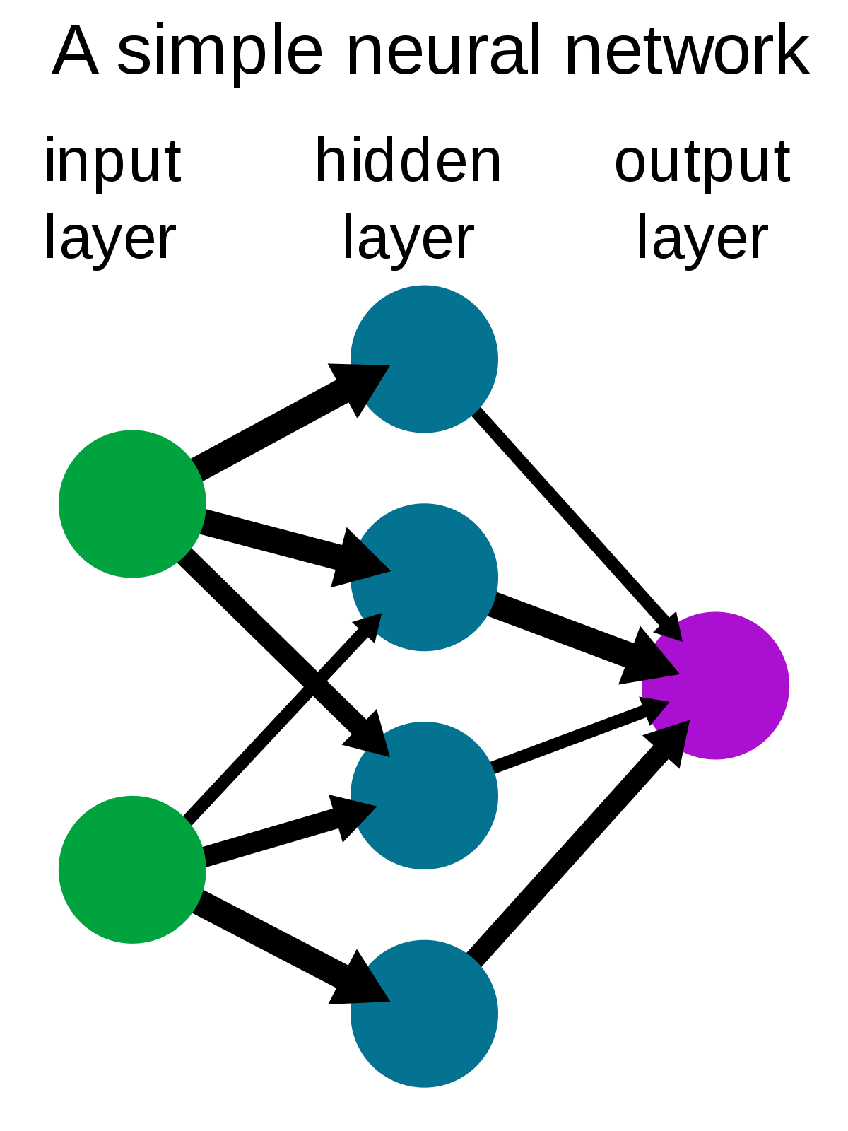
                                                                          Source: Wikipedia

Input Layer: Also known as Input nodes are the inputs/information from the outside world is provided to the model to learn and derive conclusions from. Input nodes pass the information to the next layer i.e Hidden layer.

Hidden Layer: Hidden layer is the set of neurons where all the computations are performed on the input data. There can be any number of hidden layers in a neural network. The simplest network consists of a single hidden layer.

Output layer: The output layer is the output/conclusions of the model derived from all the computations performed. There can be single or multiple nodes in the output layer. If we have a binary classification problem the output node is 1 but in the case of multi-class classification, the output nodes can be more than 1.

Perceptron and Multi-Layer Perceptron

Perceptron is a simple form of Neural Network and consists of a single layer where all the mathematical computations are performed.

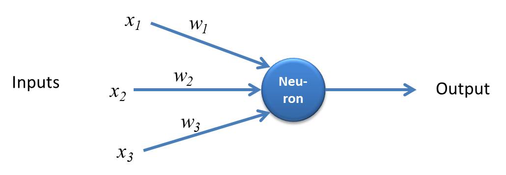
                                                         Source: kindsonthegenius.com

Whereas, Multilayer Perceptron also known as Artificial Neural Networks consists of more than one perception which is grouped together to form a multiple layer neural network.

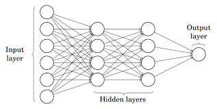
                                                                       Source: Medium

In the above image, The Artificial Neural Network consists of four layers interconnected with each other:

• An input layer, with 6 input nodes
• Hidden Layer 1, with 4 hidden nodes/4 perceptrons
• Hidden layer 2, with 4 hidden nodes
• Output layer with 1 output node

Step by Step Working of the Artificial Neural Network 

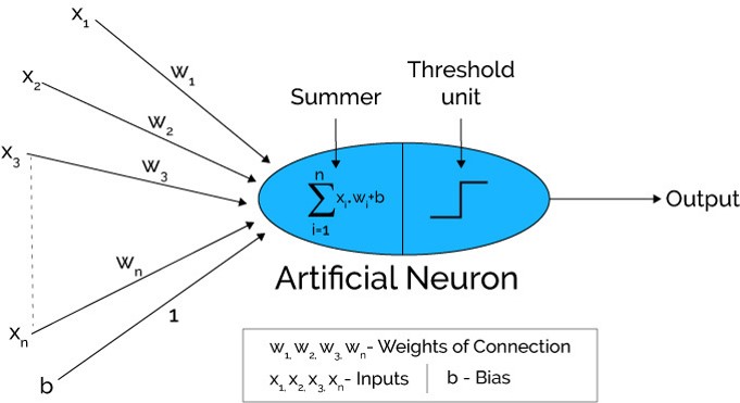
                                                                   Source: Xenonstack.com

1. In the first step, Input units are passed i.e data is passed with some weights attached to it to the hidden layer. We can have any number of hidden layers. In the above image inputs x₁,x₂,x₃,….x_n is passed.

2. Each hidden layer consists of neurons. All the inputs are connected to each neuron.

3. After passing on the inputs, all the computation is performed in the hidden layer (Blue oval in the picture)

Computation performed in hidden layers are done in two steps which are as follows :

• First of all, all the inputs are multiplied by their weights. Weight is the gradient or coefficient of each variable. It shows the strength of the particular input. After assigning the weights, a bias variable is added. Bias is a constant that helps the model to fit in the best way possible.

Z₁ = W₁*In₁ + W₂*In₂ + W₃*In₃ + W₄*In₄ + W₅*In₅ + b

W₁, W₂, W₃, W₄, W5 are the weights assigned to the inputs In₁, In₂, In₃, In₄, In_5, and b is the bias.

• Then in the second step, the activation function is applied to the linear equation Z1. The activation function is a nonlinear transformation that is applied to the input before sending it to the next layer of neurons. The importance of the activation function is to inculcate nonlinearity in the model.

There are several activation functions that will be listed in the next section.

4. The whole process described in point 3 is performed in each hidden layer. After passing through every hidden layer, we move to the last layer i.e our output layer which gives us the final output.

The process explained above is known as forwarding Propagation.

5. After getting the predictions from the output layer, the error is calculated i.e the difference between the actual and the predicted output.

If the error is large, then the steps are taken to minimize the error and for the same purpose, Back Propagation is performed.

What is Back Propagation and How it works?

Back Propagation is the process of updating and finding the optimal values of weights or coefficients which helps the model to minimize the error i.e difference between the actual and predicted values.

But here are the question is: How the weights are updated and new weights are calculated?

The weights are updated with the help of optimizers. Optimizers are the methods/ mathematical formulations to change the attributes of neural networks i.e weights to minimizer the error.

Back Propagation with Gradient Descent 

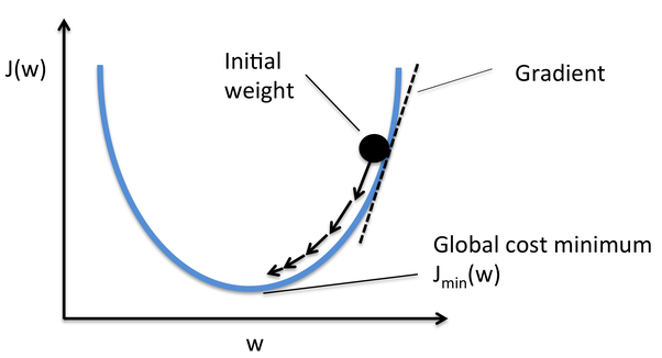
Gradient Descent is one of the optimizers which helps in calculating the new weights. Let’s understand step by step how Gradient Descent optimizes the cost function.

In the image below, the curve is our cost function curve and our aim is the minimize the error such that J_min i.e global minima is achieved.

                                                  Source: Quora

Steps to achieve the global minima:

1. First, the weights are initialized randomly i.e random value of the weight, and intercepts are assigned to the model while forward propagation and the errors are calculated after all the computation. (As discussed above)

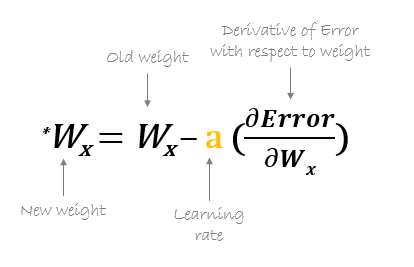
2. Then the gradient is calculated i.e derivative of error w.r.t current weights

3. Then new weights are calculated using the below formula, where a is the learning rate which is the parameter also known as step size to control the speed or steps of the backpropagation. It gives additional control on how fast we want to move on the curve to reach global minima.

                                                                   Source: hmkcode.com

       4.This process of calculating the new weights, then errors from the new weights, and then updation of weights continues till we reach global minima and loss is minimized. 

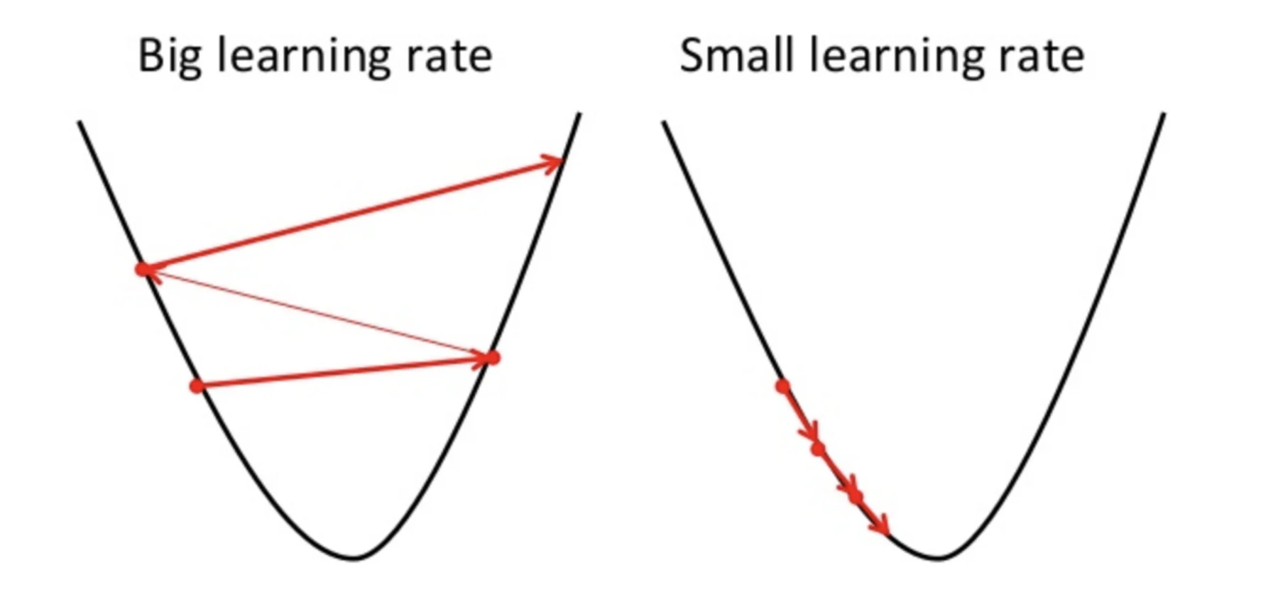
A point to note here is that the learning rate i.e a in our weight updation equation should be chosen wisely. Learning rate is the amount of change or step size taken towards reaching global minima. It should not be very small as it will take time to converge as well as it should not be very large that it doesn’t reach global minima at all. Therefore, the learning rate is the hyperparameter that we have to choose based on the model.

                                                                      Source: Educative.io

To know the detailed maths and the chain rule of Backpropagation, refer to the attached tutorial.

Brief about Activation Functions

Activation functions are attached to each neuron and are mathematical equations that determine whether a neuron should be activated or not based on whether the neuron’s input is relevant for the model’s prediction or not. The purpose of the activation function is to introduce the nonlinearity in the data.

Various Types of Activation Functions are :