Introduction
While the Transformer architecture has become the de-facto standard for natural language processing tasks, its applications to computer vision remain limited. In the vision, attention is either applied in conjunction with convolutional networks or used to replace certain components of convolutional networks while keeping their overall structure in place. We show that this reliance on CNNs is not necessary and a pure transformer can perform very well on image classification tasks when applied directly to sequences of image patches.
How many words is an image worth?
A picture is worth a thousand words? It is not possible to fully describe a picture using words. But the papers tell us that an image worth 16×16 words. In this blog, I gonna explain image recognition using transformers. It’s a really interesting paper published by Alexey Dosovitskiy, Lucas Beyer, Alexander Kolesnikov, Dirk Weissenborn, Xiaohua Zhai, Thomas Unterthiner, Mostafa Dehghani, Matthias Minderer, Georg Heigold, Sylvain Gelly, Jakob Uszkoreit, Neil Houlsby on 22 Oct 2020. In this model, authors borrowed the most dominant attention model architecture in Natural Language Processing from the paper “Attention all you need” by Ashish. In this paper, they didn’t modify the attention layers in the transformer adore. The most important trick they do is to break an image into small patches of image( perhaps 16×16 as in the title). But how these patches are divided?
What’s special about this paper?
It is special because here we won’t use any Convolutional Network Layers. It works based on a standard transformer encoder to perform image processing tasks. Transformers doesn’t have any assumptions but CNN has a lot of assumptions about the image. In fact, Transformers are originally designed for NLP. I would recommend reading the article by Jay Alammar.
Using a transformer for image processing is more challenging, in NLP we pass a sequence of tokens as input but here we pass image patches as input, fitting an image to a transformer is really challenging, but in the paper, the image is divided into small patches and passed through the transformer.
It is a simple, scalable architecture, and performs state-of-art, especially when trained on large datasets such as JFT-300M. It’s also relatively cheap to pre-train the model. Transformers completely replaced LSTM in NLP.
Self-attention to images
How to apply self-attention to images? Just like in NLP, how one word pays attention to other words ( to find the relation between the words ). Using this concept to the image, the model transformer passes one pixel to attend to every other pixel. For example, let us take an image of 4096 x 2160 pixels (DCI 4K), the computational cost too high and remember the attention layer tank capacity to the number of pixels tank capacity is high.
If you have a 1000x1M pixels image then the cost will be tremendously different. Let’s say 100×1000 pixels, the cost will be 100 times different in the self-attention layer.
How Vision Transformers work

Source – https://github.com/lucidrains/vit-pytorch/blob/main/vit.gif
Firstly, Split an image into patches. Image patches are treated as words in NLP. We have patch embedding layers that are input to transformer blocks. The sequence of pictures will have its own vectors. List of vectors as a picture because a picture is 16 times 16 words region transformer.
Vision Transformers (ViT)
As discussed earlier, an image is divided into small patches here let’s say 9, and each patch might contain 16×16 pixels. The input sequence consists of a flattened vector ( 2D to 1D ) of pixel values from a patch of size 16×16. Each flattened element is fed into a linear projection layer that will produce what they call the “Patch embedding”.
Position embeddings are then linearly added to the sequence of image patches so that the images can retain their positional information. It injects information about the relative or absolute position of the image patches in the sequence.
An extra learnable ( class) embedding is attached to the sequence according to the position of the image patch. This class embedding is used to predict the class of the input image after being updated by self-attention.
The classification is performed by just stacking an MLP Head on top of the Transformer, at the position of the extra learnable embedding that we added to the sequence.
Patch embedding

The most important part of this paper is how to break down the image into patches. An image is represented as
3D Image (X) ∈ resolution R HxWxC
reshape the 3D image into flattened 2D patches
Patch Image ( Xp) ∈ R Nx(P^2 . C)
Where sequence length N = H . W / P2 and (P, P) is the resolution of each image patch.
Each patch is a D dimension vector with a trainable linear projection.
[class] token
![[class] token Vision Transformers](https://geeksforgeeks.org/wp-content/uploads/2024/07/rubhabha_rubhabha_27194class.jpg)
Similar to BERT’s [class] token, we prepend a learnable embedding to the sequence of embedded patches (z00 = xclass ).
z0 = [xclass; x1pE; x2pE; · · · ; xNp E] + Epos, E ∈ R(P^2C)×D, Epos ∈ R(N+1)×D
Xclass is a class label and XNp is patch images N ∈ 1 to n
Using the transformer encoder to pre-train we always need a Class label at the 0th position. When we pass the patch images as inputs we always need to prepend one classification token as the first patch as shown in the figure.
Positional encodings / Embeddings
Since Transformers need to learn the inductive biases for the task they are being trained for, it is always beneficial to help that learning process by all means. Any inductive bias that we can include in the inputs of the model will facilitate its learning and improve the results.
Position embeddings are added to the patch embeddings to retain positional information. In Computer Vision, these embeddings can represent either the position of a feature in a 1-dimensional flattened sequence or they can represent a 2-dimensional position of a feature.
1-dimensional: a sequence of patches, works better
2-dimensional: X-embedding and Y-embedding
Relative: Define the relative distance of all possible pairs.

Position Embedding formula as per attention mechanism
Model architecture
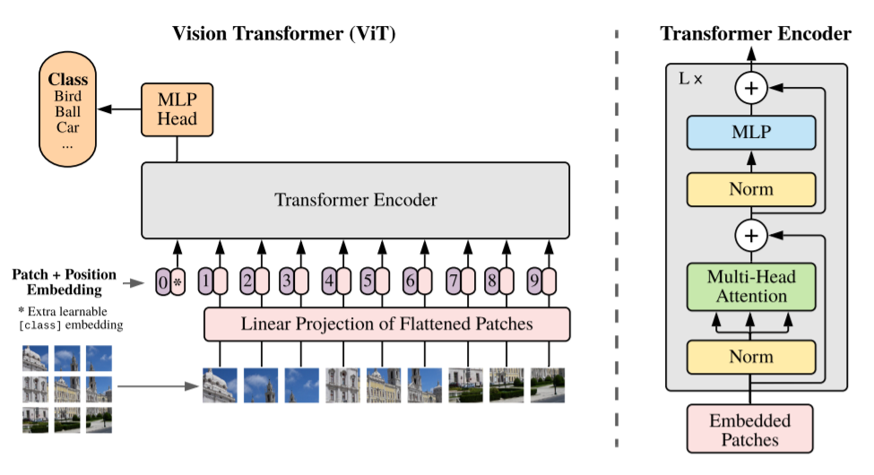
Image is from From paper
If we do not provide the transformer with the positional information, it will have no idea of the images’ sequence (which comes first and the images that follow it). This sequence of vector images is then fed into the transformer encoder.
The Transformer encoder module comprises a Multi-Head Self Attention ( MSA ) layer and a Multi-Layer Perceptron (MLP) layer. The Multi-Head Self Attention layer split inputs into several heads so that each head can learn different levels of self-attention. The outputs of all the heads are then concatenated and passed through the Multi-Layer Perceptron.
Layernorm (LN) is applied before
every block, and residual connections after every block.The MLP contains two layers with a GELU non-linearity. Finally, an extra learnable classification module (the MLP Head) is added to the transformer encoder, giving the network’s output classes.
GELU is GAUSSIAN ERROR LINEAR UNIT
zℓ ` = MSA(LN(zℓ−1)) + zℓ−1, ℓ = 1 . . . L
zℓ = MLP(LN(zℓ `)) + zℓ ` ℓ = 1 . . . L
y = LN(z0L) ==> Transformer encoder (z0L) serves as theimage representation y

Hybrid architecture
As an alternative to raw image patches, the input sequence can be formed from feature maps of a CNN. In this hybrid model, the patch embedding
projection (E ) is applied to patches extracted from a CNN feature map. As a special case, the patches can have spatial size 1×1 ( 1 pixel ), which means that the input sequence is obtained by simply flattening the spatial dimensions of the feature map and projecting to the Transformer dimension.
The classification input embedding and position embeddings are added as described above.
E = [xclass; x 1pE; x 2pE; · · · ; x Np E] + Epos, E ∈ R (P^2 ·C)×D, Epos ∈ R (N+1)×D
Fine-tuning and Higher resolution
Supervised learning is used to do pretraining on large datasets ( e.x.; ImageNet). Pre-trained prediction head and attached a zero-initialized D × K feedforward layer, where K is the number of downstream classes ( e.x; 10 downstream classes in ImageNet ).
On higher resolution images, It is often beneficial to fine-tune at a higher resolution than pre-training. When feeding images of higher resolution, we keep the patch size the same, which results in a larger effective sequence
length.
The Vision Transformers can handle arbitrary sequence lengths (up to memory constraints), however, if sequence lengths too long the pre-trained position embeddings may no longer be meaningful.
2D interpolation of the pre-trained position embeddings is performed, according to their location in the original image. Note that this resolution adjustment and patch extraction are the only points at which an inductive bias about the 2D structure of the images is manually injected into the Vision Transformers.
Datasets
|
The authors of the paper have trained the Vision Transformer on a private Google JFT-300M dataset containing 300 million (!) images, which resulted in state-of-the-art accuracy on a number of benchmarks ( Image below).
Model variants
| Model |
Layers |
Hidden size D |
MLP size |
Heads |
Params |
| ViT-Base | 12 | 768 | 3072 | 12 | 86M |
| ViT-Large | 24 | 1024 | 4096 | 16 | 307M |
| ViT-Huge | 32 | 1280 | 5120 | 16 | 632M |
Details of Vision Transformer model variants
The “Base” and “Large” models are directly adopted from BERT and the larger “Huge” models. For instance, ViT-L/16 means the “Large” variant with 16×16 input patch size. The transformer’s sequence length is inversely proportional to the square of the patch size, thus models with smaller patch size are computationally more expensive.
Comparison to state-of-the-art

Models – ViT-H/14 and ViT-L/16 – to state-of-the-art CNNs from the literature. Big Transfer (BiT) , which performs supervised transfer learning with large ResNets and Noisy Student, which is a large EfficientNet trained using semi-supervised learning on ImageNet and JFT300M with the labels removed. Currently, Noisy Student is the state of the art on ImageNet and BiT-L on the other datasets reported here. All models were trained on TPUv3 hardware, and less number of TPUv3-core-days ( 2500 TPU days ) taken to pre-train each of them.
Model size vs data size
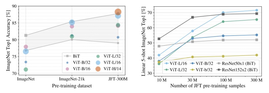
ImageNet, Imagenet-21, and JFT-300 datasets are small, medium, and huge respectively. For the small dataset, Resnet ( Bit) really performed well but as we scale up the dataset ViT is performing very well. Vision Transformer performed very well on JFT-300 dataset. Localization is implemented on a very huge dataset during training. Localization like learning rate decay, dropout, and SGD with momentum.
ResNets perform better with smaller pre-training datasets but plateau sooner than ViT, which performs better with larger pre-training. ViT-b is ViT-B with all hidden dimensions halved.
Scaling Data Study
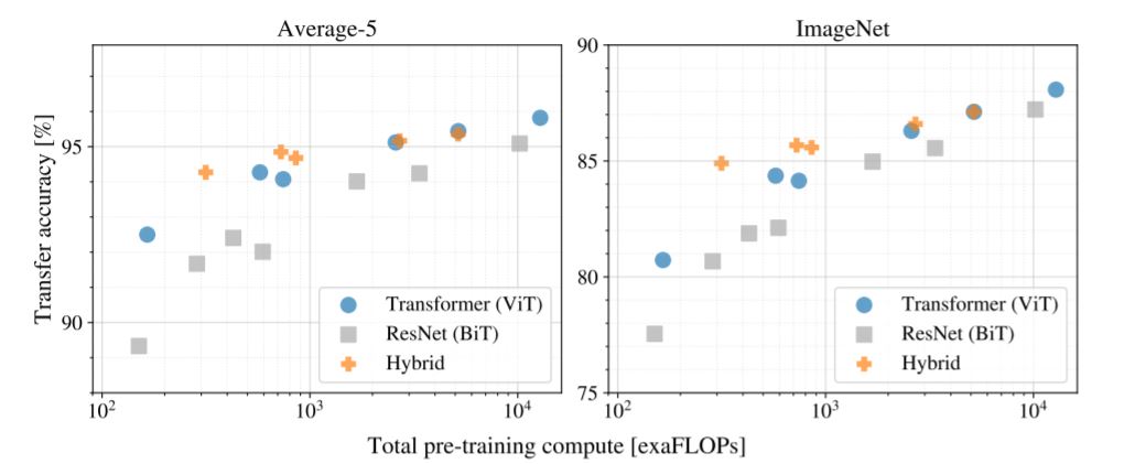
The above figure shows, transfer performance versus total pre-training compute/computational costs. A few patterns can be observed.
First, Vision Transformers dominate ResNets on the performance/compute trade-off. ViT uses approximately 2 − 4× less compute to attain the same
performance (average over 5 datasets).
Second, hybrids slightly outperform ViT at small computational budgets, but the difference vanishes for larger models. This result is somewhat surprising since one might expect convolutional local feature processing to assist ViT at any size.
Third, Vision Transformers appear not to saturate within the range tried, motivating future scaling efforts.
Attention heads and distance over layers
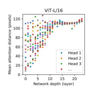
How transformer pays attention when processing an image, to understand how ViT uses self-attention to integrate information across the image, authors analyzed the average distance spanned by attention weights at different layers. This “attention distance” is analogous to receptive field size in CNNs. Average attention distance is highly variable across heads in lower layers, with some heads attending too much of the image, while others attend to small regions at or near the query location. As depth increases, attention distance increases for all heads. In the second half of the network, most heads attend widely across tokens.
Attention pattern analysis
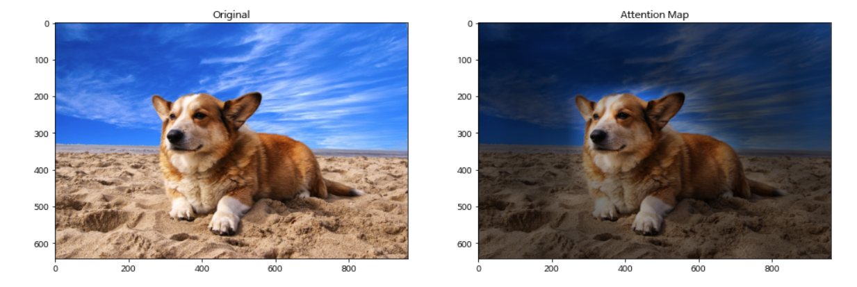
I would suggest reading “Attention is all you need” article by Jay Alamar. A representative example of attention from the output token to the input
space. Average attention weights of all heads mean heads across layers and the head in the same layer. So, basically, the area has every attention in the transformer, this is called attention pattern or attention matrix.
When the patch image is passed through the transformer, the transformer will generate the attention weights matrix for the image patches. When patch-1 is passed through the transformer, self-attention will calculate how much attention should pay to others ( Patch 2, Patch 3,….). And every head will have one attention pattern like shown in the image and finally, they will sum up all attention patterns ( all heads )to get the above picture.
Self-supervised pre-training
Transformers show impressive performance on NLP tasks. However, much of their success stems
not only from their excellent scalability but also from large-scale self-supervised pre-training. We also perform a preliminary exploration on masked patch
prediction for self-supervision, mimicking the masked language modeling task used in BERT. With
self-supervised pre-training, our smaller ViT-B/16 model achieves 79.9% accuracy on ImageNet, a
significant improvement of 2% to training from scratch, but still 4% behind supervised pre-training. We leave the exploration of contrastive pre-training to future work.
Summary / Conclusion
- Transformers solve a problem that was not only limited to NLP, but also to Computer Vision tasks.
- Huge models (ViT-H) generally do better than large models (ViT-L) and wins against state-of-the-art methods.
- Vision transformers work better on large-scale data.
- Attention Rollouts are used to compute the attention maps.
- Like the GPT-3 and BERT models, the Visual Transformer model also can scale.
- Large-scale training outperforms inductive bias.
- Convolutions are translation invariant, locality-sensitive, and lack a global understanding of images
So does this mean that CNNs are extinct? No! CNN still very much effective for tasks like object detection and image classification. As ViT works on large datasets, so we can make use of ResNet and EfficientNet models which are state-of-the-art convolutional architectures for all types (small, medium, and large )datasets. However, transformers have been a breakthrough in natural language processing tasks such as language translation and show quite a promise in the field of computer vision.
Please do share if you like my post.
Reference
- https://www.youtube.com/watch?v=Gl48KciWZp0&t=1539s
- https://arxiv.org/pdf/2010.11929.pdf
- https://towardsdatascience.com/transformers-in-computer-vision-farewell-convolutions-f083da6ef8ab
- Images are taken from Google Images and published papers.
The media shown in this article are not owned by Analytics Vidhya and is used at the Author’s discretion.


