All you need to know about Convolutional Neural Networks!

This article was published as a part of the Data Science Blogathon

Table of Contents:

1. What is CNN, Why is it important

2. Biological Inspiration

3. Fundamentals of CNN

4. Various Convolutional Neural Networks

5. Data Augmentation and Transfer Learning

6. Code example using Keras

What is CNN, Why is it important

Ever since I learned about CNN, it has become one of my favorite topics in Deep Learning, so in this article, I am going to explain everything related to CNN. “Using this we can provide machines with vision. Now vision, I believe is one of the most important senses that we pose. Sighted people rely on vision for everyday tasks such as navigation, recognize objects, recognize complex human emotions and behavior” these are some of the words of Professor Alexander Amini from ‘MIT Introduction to Deep Learning 6.S191’. Since CNN has been specifically designed for visual tasks (say object recognition) so I can say that CNN is a type of Neural Network that is most often applied to image processing problems.

It can be used to detect and recognize faces, can be used in the medical sector to classify various diseases instantly, another example where CNN can be used is autonomous/self-driving cars.

Biological Inspiration

Photo by MIKHAIL VASILYEV on Unsplash

Let’s try to understand this from the historical perspective first. Hubel and Wiesel, two neuroscientists who got their Nobel prize in medicine mostly focused their research on visual tasks, so in an experiment done in 1959, they anesthetized a cat and inserted a microelectrode into its primary visual cortex. They then project a series of light bars on the screen installed in front of the cat. Interestingly they observed that some neurons showed some activity when this light bar was presented at a specific angle while other neurons got activated to some different angle of light bars. What they found was that there were different neurons for different tasks such as edge detection, motion detection, depth detection, and so on. CNN is inspired by this biological idea and research done on this area.

Having known the basic idea of CNN le us try to understand it in more detail.

Fundamentals of CNN

1. Convolution

As you might have guessed from the name itself convolution convols/merge two functions or information to produce a third function/information.

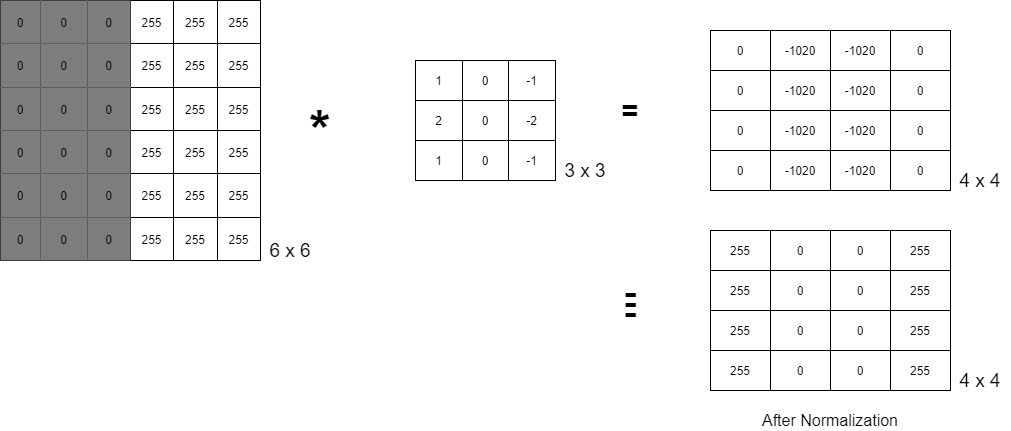
Let’s consider this gray-scaled image of 6×6 dimensions. Since the machine can only understand binary language, this image would appear to be a 6×6 matrix with all 0s on the left half and all 255 on the right half, since it is a grayscale image. The RHS 3×3 matrix is known as kernel/ filter/ mask/ operator, and the * operator is a convolution operator (here it is Sobel edge detector). We now have a 4×4 matrix after doing component-wise multiplication and addition. When we normalize this matrix, we receive an image with an edge highlighted in it.

Formula – (n x n) * (k x k) => (n – k + 1) x (n – k + 1)

2. Padding (p)

 

What if we want the output matrix to have the same dimensions as the input matrix i.e. (nxn). If you substitute n = 6 from the above formula, you will get an output matrix of size 4×4. If you want the output matrix to be of size 6×6 then it is quite obvious that the input matrix should be of size 8×8, so to change the dimensions of the input matrix, there is a concept of padding. If a pad one extra layer to each side then the initial dimension would be increased by 2 i.e. now n = 8 which will give the output matrix dimension to be 6.

Now the question arises what value should I fill this extra layer with?

There are two approaches to it:

1. Zero – Padding

2. Same-value Padding

Now the above formula becomes (n x n) * (k x k) with padding ‘p’ => (n – k + 2p + 1) x (n – k + 2p + 1)

3. Stride (s)

Basically, the stride is nothing but shifting a kernel matrix over the input matrix by a specific number of cells at a time. It helps to reduce the size of the output matrix.

Formula – (n x n) * (k x k) with stride = ‘s’ => ((n – k) // s + 1) x ((n – k) // s + 1)

Finally, the formula combining all these would be: (n x n) * (k x k), padding = p, stride = s ⇒ (((n – k + 2p) // s) + 1) x (((n – k + 2p) // s) + 1)

NOTE: Here // (written in python) is equivalent to the mathematical floor value after division.

Convolution in Color Images

So far we have looked at the convolution operation, padding, and stride on a greyscale image, what if the image is a colorful image? A color image can be represented as a 3D tensor since it has 3 matrices of Red, Green, and Blue stacked on top of each other. These RGB matrices are often referred to as 3 channels since most of the concepts in image processing are derived from signal processing in electronics and telecommunications major. Hence we can represent this 3D tensor as NxMxC where C is the no. of channels which is equal to 3 for color images.

Similar to the convolution in 2D matrices, convolution in 3D matrices is also component-wise multiplication followed by addition. One thing to keep in mind here is that the kernel should also have the same number of channels as the input matrix.

Formula: (N x N x C) * (K x K x C) ⇒ (N – K + 1) x (N – K + 1) x 1

NOTE: Convolution of a 3D matrix results in a 2D matrix.

Convolution layer

Unlike image processing where we use predefined kernels like the Sobel edge detector, in CNN we try to learn these kernels.

Here in CNN, we have multiple hyperparameters to play with, like kernel size K, padding p, stride s, and the number of kernels M.

In a real-world scenario, we have a series of convolution layers to train first the low-level features like edges, then mid-level features, then high-level features to get a fairly accurate model.

Max-pooling

It is again a biologically inspired concept that introduces some invariance in the model. For example, the model should be in a position to detect a face in an input image no matter where it is located and no matter what its size is. This is achieved using pooling layers.

This is similar to the kernel we have seen above, here also we can apply the concept of strides, kernel size, etc.

Here in this example, we have a 2 x 2 max-pool kernel with stride as 2. It selects the maximum value from a patch. Another pooling is the mean/average pooling where we get the average value instead of the maximum value.

Various Convolutional Neural Networks:

• LeNet, 1998

• AlexNet, 2012

• VGGNet, 2014

• ResNet, 2015

• Inception Network, 2015

Before we move on to the code part, it is important that we understand what Data Augmentation and Transfer Learning mean.

Data Augmentation

Since everyone wants their model to be a robust model but creating such a model would require a huge amount of data so Data Augmentation comes to the rescue here. It basically means adding more data to our dataset by rotating, scaling, cropping, flipping, shifting horizontally or vertically, zooming, stretching (shear operation), illumination conditions, etc on images (since CNN) to create more artificial data to train on.

Transfer Learning

The main idea is to use a pre-trained model (which is trained on some dataset ‘X) on a dataset ‘Y’ without training it from scratch. Both in Keras and Tensorflow we have some pre-trained models like VGG16 that is trained on one of the largest object classification datasets ImageNet contained 1000 different categories and the total dataset size is 150GB.

Here we can use transfer learning in various ways like using Bottleneck features (i.e. taking output just at the flattening layer) or by freezing the initial layer that detects only edges, shapes, etc. and changing/learning the last few layers according to the new dataset or use the pre-trained model as the initial model to fine-tune the complete model based on the new dataset.

Let’s Code

from __future__ import print_function
import keras
from keras.datasets import mnist
from keras.models import Sequential
from keras.layers import Dense, Dropout, Flatten
from keras.layers import Conv2D, MaxPooling2D
from keras import backend as K
batch_size = 128
num_classes = 10
epochs = 12
# input image dimensions
img_rows, img_cols = 28, 28
# the data, split between train and test sets
(x_train, y_train), (x_test, y_test) = mnist.load_data()
if K.image_data_format() == 'channels_first':
    x_train = x_train.reshape(x_train.shape[0], 1, img_rows, img_cols)
    x_test = x_test.reshape(x_test.shape[0], 1, img_rows, img_cols)
    input_shape = (1, img_rows, img_cols)
else:
    x_train = x_train.reshape(x_train.shape[0], img_rows, img_cols, 1)
    x_test = x_test.reshape(x_test.shape[0], img_rows, img_cols, 1)
    input_shape = (img_rows, img_cols, 1)
x_train = x_train.astype('float32')
x_test = x_test.astype('float32')
x_train /= 255
x_test /= 255
print('x_train shape:', x_train.shape)
print(x_train.shape[0], 'train samples')
print(x_test.shape[0], 'test samples')
# convert class vectors to binary class matrices
y_train = keras.utils.to_categorical(y_train, num_classes)
y_test = keras.utils.to_categorical(y_test, num_classes)
model = Sequential()
model.add(Conv2D(32, kernel_size=(3, 3),
                 activation='relu',
                 input_shape=input_shape))
model.add(Conv2D(64, (3, 3), activation='relu'))
model.add(MaxPooling2D(pool_size=(2, 2)))
model.add(Dropout(0.25))
model.add(Flatten())
model.add(Dense(128, activation='relu'))
model.add(Dropout(0.5))
model.add(Dense(num_classes, activation='softmax'))
model.compile(loss=keras.losses.categorical_crossentropy,
              optimizer=keras.optimizers.Adadelta(),
              metrics=['accuracy'])
model.fit(x_train, y_train,
          batch_size=batch_size,
          epochs=epochs,
          verbose=1,
          validation_data=(x_test, y_test))
score = model.evaluate(x_test, y_test, verbose=0)
print('Test loss:', score[0])
print('Test accuracy:', score[1])

References

1. https://towardsdatascience.com/covolutional-neural-network-cb0883dd6529

2. https://towardsdatascience.com/a-comprehensive-guide-to-convolutional-neural-networks-the-eli5-way-3bd2b1164a53

3. https://www.youtube.com/watch?v=iaSUYvmCekI

4. https://github.com/keras-team/keras/blob/master/examples/mnist_cnn.py

The media shown in this article are not owned by Analytics Vidhya and are used at the Author’s discretion.