A Detailed Study of Self Supervised Contrastive Loss and Supervised Contrastive Loss

Introduction

Supervised Contrastive Learning paper claims a big deal about supervised learning and cross-entropy loss vs supervised contrastive loss for better image representation and classification tasks. Let’s go in-depth in this paper what is about.

Claim actually close to 1% improvement on image net data set¹.

Architecture wise, its a very simple network resnet 50 having a 128-dimensional head. If you want you can add a few more layers as well.

Codeself.encoder = resnet50()self.head = nn.Linear(2048, 128)def forward(self, x):
 feat = self.encoder(x)
 #normalizing the 128 vector is required
 feat = F.normalize(self.head(feat), dim=1)
 return feat

As shown in the figure training is done in two-stage.

• Train using contrastive loss (two variations)
• freeze the learned representations and then learn a classifier on a linear layer using a softmax loss. (From the paper)

The above is pretty self explanatory.

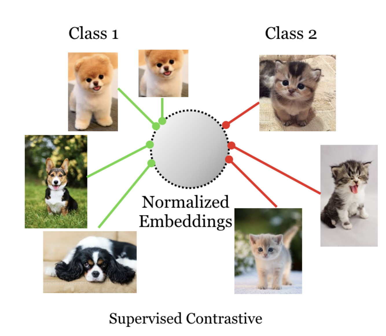
Loss, the main flavor of this paper is understanding the self-supervised contrastive loss and supervised contrastive loss.

As you can see from the above diagram¹ in SCL (supervised contrastive Loss), a cat is contrasted with any noncat. which means all cats belong to the same label and work as a positive pair and anything noncat is negative. This is very similar to triplet Data and how triplet loss² works.

In case you confused every cat images will be augmented also every-time so even from a single cat image we will have lots of cats.

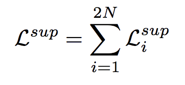
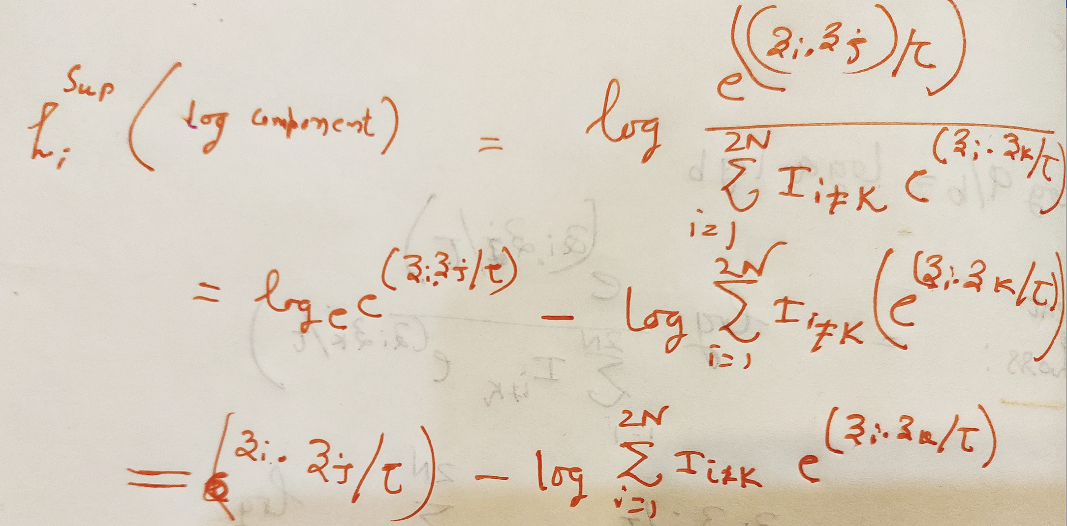
Loss Function for supervised contrastive loss, although it looks monster it’s actually quite simple.

We will see some code later but first very simple explanation. every z is 128 dimensional vector which are normalised.

which means ||z|| =1
Just to reiterate fact from Linear Algebra if u and v two vectors are normalised implies u.v = cos(angel between u and v)
which means if two normalised vector are same the dot product between them = 1
# try the below code to convince your selfimport numpy as np
v = np.random.randn(128)
v = v/np.linalg.norm(v)
print(np.dot(v,v))
print(np.linalg.norm(v))

The loss function is with the assumption that every image has one augmentation, N images in a batch create a batch size = 2*N

Read the section of the paper “Generalisation to an arbitrary number of positives”¹

Numerator exp(z_i.z_j)/tau is a representation of all cats in a batch. Take dot product of z_i which is the 128 dim vector of i^th image representation with all the j^th 128 dim vectors such that their label is the same and i!=j.

The denominator is i^th cat image is dotted with everything else as long it’s not the same cat image. Take the dot of z_i and z_k such that i!=k means it’s dotted with every image except itself.

Finally, we take the log probability and sum it overall cat images in the batch except itself and divide by 2*N-1

Total Loss sum of losses for all images

Code Let’s understand the above using some torch code.

Let’s assume our batch size is 4 and let’s see how to calculate this loss for a single batch.

For a batch size of 4, your input to the network will be 8x3x224x224 where I have taken image width and height 224.

The reason for 8 = 4X2 as we always have one contrast for each image, one needs to write a data loader accordingly.

The Super contrastive resnet will output you a dimension 8×128 lets split those properly for calculating the batch loss.

#batch_size
bs = 4

Numerator Code lets calculate this part

temperature = 0.07anchor_feature = contrast_feature#Note we not doing exp their is a reason see below
anchor_dot_contrast = torch.div(
    torch.matmul(anchor_feature, contrast_feature.T),
    temperature)

Anchor Dot Contrast in case you confused, our feature shapes are 8×128, lets take a 3×128 matrix and the transpose of that and dot them, see the below picture if you can visualize.

anchor_feature = 3×128 contrast_feature = 128×3 result is 3×3 as below

If you notice all diagonal elements are dot with themselves which we don’t want we will get rid of them next.

Linear Algebra fact if u and v are two vectors then u.v is maximum when u = v. So in each row if we take the max of anchor_dot_contrast and negate the same all diagonal will become 0.

Let’s drop the dimension from 128 to 2 to better see this and batch size of 1.

#resnet output just mind you i am not normalizing but according to paper you need to use normalize look into torch Functional.#bs 1 and dim 2 means 2*1x2 
features = torch.randn(2, 2)temperature = 0.07 
contrast_feature  = features
anchor_feature = contrast_feature
anchor_dot_contrast = torch.div(
    torch.matmul(anchor_feature, contrast_feature.T),
    temperature)
print('anchor_dot_contrast=\n{}'.format(anchor_dot_contrast))logits_max, _ = torch.max(anchor_dot_contrast, dim=1, keepdim=True)
print('logits_max = {}'.format(logits_max))
logits = anchor_dot_contrast - logits_max.detach()
print(' logits = {}'.format(logits))#output see what happen to diagonalanchor_dot_contrast=
tensor([[128.8697, -12.0467],
        [-12.0467,  50.5816]])
 logits_max = tensor([[128.8697],
        [ 50.5816]])
 logits = tensor([[   0.0000, -140.9164],
        [ -62.6283,    0.0000]])

Mask. Artificial label creation and creating an appropriate mask for contrastive calculation. This code is a little tricky, so check the output carefully.

bs = 4
print('batch size', bs)
temperature = 0.07
labels = torch.randint(4, (1,4))
print('labels', labels)
mask = torch.eq(labels, labels.T).float()
print('mask = \n{}'.format(logits_mask))#hard coding it for easier understanding otherwise its features.shape[1]
contrast_count = 2
anchor_count = contrast_countmask = mask.repeat(anchor_count, contrast_count)# mask-out self-contrast cases
logits_mask = torch.scatter(
    torch.ones_like(mask),
    1,
    torch.arange(bs * anchor_count).view(-1, 1),
    0
)
mask = mask * logits_mask
print('mask * logits_mask = \n{}'.format(mask))

 Let’s understand the output.

batch size 4
labels tensor([[3, 0, 2, 3]])#what above means in this perticuler batch of 4 we got 3,0,2,3 labels. Just in case you forgot we are contrasting here only once so we will have 3_c, 0_c, 2_c, 3_c as our contrast in the input batch.
#basically batch_size X contrast_count X C x Width X height -> check above if you confusedmask = 
tensor([[0., 1., 1., 1., 1., 1., 1., 1.],
        [1., 0., 1., 1., 1., 1., 1., 1.],
        [1., 1., 0., 1., 1., 1., 1., 1.],
        [1., 1., 1., 0., 1., 1., 1., 1.],
        [1., 1., 1., 1., 0., 1., 1., 1.],Easy to understand the Self Supervised Contrastive Loss now which is simpler than this.
        [1., 1., 1., 1., 1., 0., 1., 1.],
        [1., 1., 1., 1., 1., 1., 0., 1.],
        [1., 1., 1., 1., 1., 1., 1., 0.]])#this is really important so we created a mask = mask * logits_mask which tells us for 0 th image representation which are the image it should be contrasted with.# so our labels are labels tensor([[3, 0, 2, 3]])
# I am renaming them for better understanding tensor([[3_1, 0_1, 2_1, 3_2]])
# so at 3_0 will be contrasted with its own augmentation which is at position 5 (index = 4) and position 8 (index = 7) in the first row those are the position marked one else its zero
See the image bellow for better understandingmask * logits_mask = 
tensor([[0., 0., 0., 1., 1., 0., 0., 1.],
        [0., 0., 0., 0., 0., 1., 0., 0.],
        [0., 0., 0., 0., 0., 0., 1., 0.],
        [1., 0., 0., 0., 1., 0., 0., 1.],
        [1., 0., 0., 1., 0., 0., 0., 1.],
        [0., 1., 0., 0., 0., 0., 0., 0.],
        [0., 0., 1., 0., 0., 0., 0., 0.],
        [1., 0., 0., 1., 1., 0., 0., 0.]])

Anchor dot contrast if you remember from above as below.

logits = anchor_dot_contrast — logits_max.detach()

Loss again

Math recap

We already have the first part dot product divided by tau as logits.

#second part of the above equation equal to torch.log(exp_logits.sum(1, keepdim=True))exp_logits = torch.exp(logits) * logits_mask
log_prob = logits - torch.log(exp_logits.sum(1, keepdim=True))# compute mean of log-likelihood over positive
mean_log_prob_pos = (mask * log_prob).sum(1) / mask.sum(1)# loss
loss = - mean_log_prob_posloss = loss.view(anchor_count, 4).mean()
print('19. loss {}'.format(loss))

I think that’s about the supervised contrastive loss. I think it’s very easy to understand the Self Supervised Contrastive Loss now which is simpler than this.

According to the paper, more contrast_count makes a better model which is self-explanatory. Need to modify the loss function for more than 2 contrast count, hope you can try it with the help of the above explanation.

References

• [1] : Supervised Contrastive Learning
• [2] : Florian Schroff, Dmitry Kalenichenko, and James Philbin. Facenet: A unified embedding for face recognition and clustering. In Proceedings of the IEEE conference on computer vision and pattern recognition, pages 815–823, 2015.
• [3] : A Simple Framework for Contrastive Learning of Visual Representations, Ting Chen, Simon Kornblith, Mohammad Norouzi, Geoffrey Hinton
• [4] : https://github.com/google-research/simclr

About the Author