Introduction
This article briefly introduces Image thresholding and the algorithms used for image thresholding. Image thresholding is a simple image segmentation technique. It is used to convert a grayscale image or RGB image to a binary image. In this article, we will look into thresholding algorithms like simple thresholding, otsu’s thresholding, and adaptive thresholding technique, along with a brief note on a deep learning algorithm (U-Net) for image segmentation.
What is Image Thresholding?
Before understanding the term Image Thresholding, let us first understand the term Image Segmentation. Image segmentation is a common technique used to divide an image into groups of pixels based on some criteria.
Image thresholding is a type of image segmentation that divides the foreground from the background in an image. In this technique, the pixel values are assigned corresponding to the provided threshold values. In computer vision, thresholding is done in grayscale images.
The below images show a grayscale image and the image obtained after applying thresholding on it.
Why do we need Image Thresholding?
Let us understand the importance of image thresholding with an example-
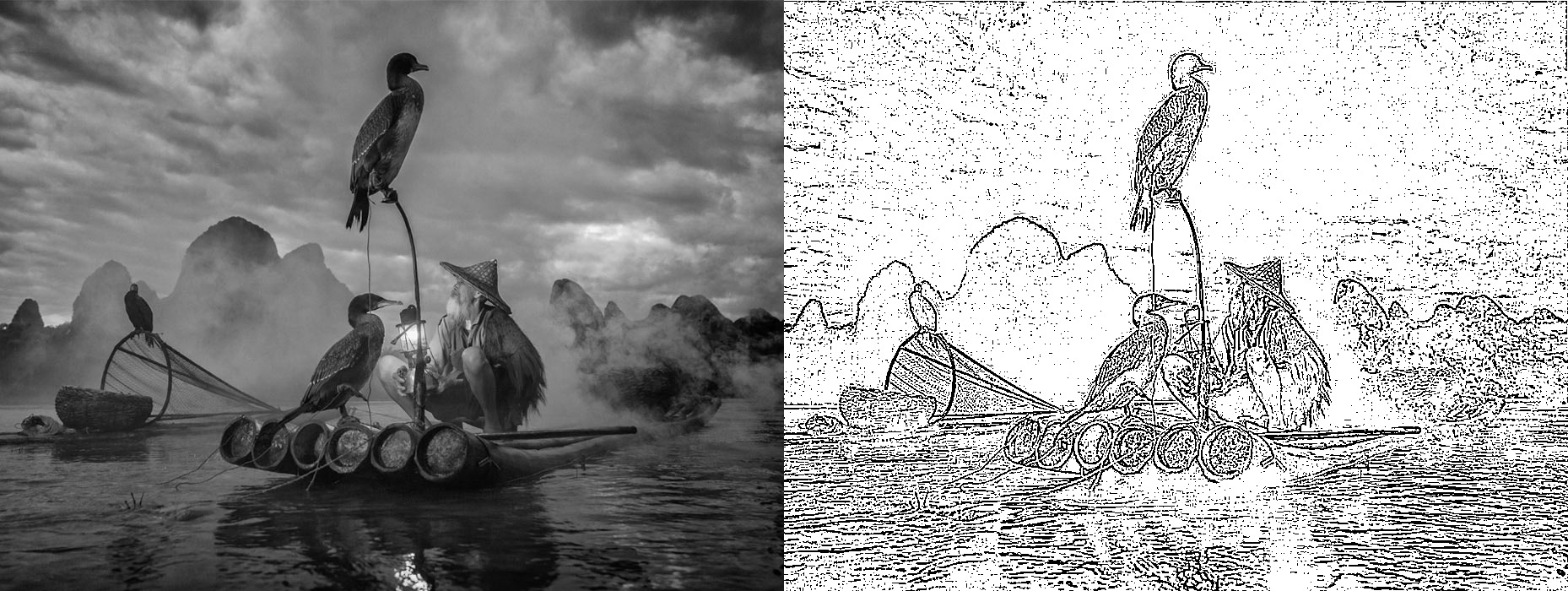
Take a look at the images below,
Comparing the first image, the mask in the second image is visible clearly. Let’s take another example,
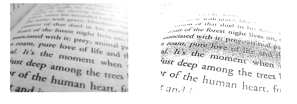
The first image, the original image, is a little distorted than the second image we obtained after applying thresholding. So thresholding is useful in extracting text that is not clear in the image.
Image thresholding helps us divide an image’s foreground and background, which can help to identify the objects that are not clearly visible in the images.
Understanding different thresholding techniques
In this article, we will learn about different techniques used in image thresholding and implement those techniques using OpenCV.
Simple Thresholding
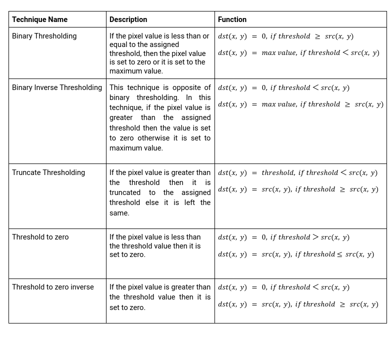
Simple Thresholding is also known as Binary thresholding. This technique sets a threshold value and compares each pixel to that particular threshold value. If the pixel value is less than or equal to the assigned threshold, then the pixel value is set to zero or to the maximum value.
Implementation of Simple Thresholding using OpenCV:
Importing necessary libraries
import cv2
from google.colab.patches import cv2_imshow
import matplotlib.pyplot as plt
Converting a color image into grayscale
image = cv2.imread('/content/drive/MyDrive/AV/OpenCV/test.jpg')
cv2_imshow(image)
# coverting color image into grayscale
orig_img = cv2.cvtColor(image, cv2.COLOR_BGR2GRAY)
Binary Thresholding
# Arguments of function cv2.threshold
# cv2.threshold(grayscaled image, threshold value, maximum value of pixel, type of threshold)
# Output is a tuple containg the threshold value and thresholded image

t, thresh = cv2.threshold(orig_img,70,255,cv2.THRESH_BINARY)
cv2_imshow(thresh)
Binary Inverse Thresholding
t,thresh1 = cv2.threshold(orig_img,70,255,cv2.THRESH_BINARY_INV)
cv2_imshow(thresh1)
Truncate Thresholding
rect,thresh2 = cv2.threshold(orig_img,70,255,cv2.THRESH_TRUNC)
cv2_imshow(thresh2)
Threshold to zero
rect,thresh3 = cv2.threshold(orig_img,70,255,cv2.THRESH_TOZERO)
cv2_imshow(thresh3)
Threshold to zero inverse
rect,thresh4 = cv2.threshold(orig_img,127,255,cv2.THRESH_TOZERO_INV)
cv2_imshow(thresh4)
The below image is obtained after applying simple thresholding
Otsu’s Thresholding
One of the ways to achieve an optimal threshold is Otsu’s method. In this method, we find the spread of foreground and background of the pictures for all possible values of threshold. The threshold with the least spread is taken as the optimal threshold.
How does Otsu’s thresholding work?
The idea in Otsu’s thresholding is to maximize the between-class variance. The between-class variance can be defined as follows,
Here, is the between-class variance of two classes – foreground class and background class.
Let, be the number of pixels in the background and foreground classes, respectively. n the total number of pixels in the image then,
The mean of background class and foreground class is represented as
Otsu’s algorithm calculates the between-class variance for all possible threshold values. The threshold with the highest between-class variance is taken as the optimal threshold value. Values less than the optimal threshold value falls into one class and other values fall into another class.
Implementation of Otsu’s Thresholding:
Implementation of Otsu’s Thresholding using OpenCV
blur = cv2.GaussianBlur(orig_img,(5,5),0) #Applying Gaussian Blurr on image to get better threshold

t,thresh5 = cv2.threshold(blur,128,255,cv2.THRESH_BINARY+cv2.THRESH_OTSU)
print('Threshold obtained by Otsu Thresholding : ', t)
cv2_imshow(thresh5)
The below image was obtained after applying Otsu’s binarization thresholding.
Adaptive Thresholding
Both Simple thresholding and Otsu’s thresholding are global thresholding techniques using a single threshold value in image thresholding. But a single threshold value may not be sufficient because it may work well in a certain part of the image but may fail in another part. To resolve these limitations, adaptive thresholding can be used.
Adaptive thresholding is a local thresholding technique. This technique considers each pixel and its neighborhood. The arithmetic mean or Gaussian mean of pixels intensity is commonly used to calculate the threshold of the neighborhood; then the threshold value is used to classify the pixel. In Gaussian mean, pixel value farther from the center of the region contributes less in finding the threshold of the region, while in arithmetic mean, all pixel values contribute equally.
Implementation of Adaptive thresholding using OpenCV:
# Arithmatic Mean Adaptive thresholding

thresh6 = cv2.adaptiveThreshold(orig_img,255,cv2.ADAPTIVE_THRESH_MEAN_C,cv2.THRESH_BINARY,5,4)
cv2_imshow(thresh6)
# Gaussian Mean Thresholding

thresh7 = cv2.adaptiveThreshold(orig_img,255,cv2.ADAPTIVE_THRESH_GAUSSIAN_C,cv2.THRESH_BINARY,5,4)
cv2_imshow(thresh7)
The below images were obtained after applying adaptive thresholding:
Introduction to UNet: Deep learning Model for Image Segmentation
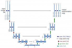
In this article, we will be discussing U-Net Architecture for Image segmentation. The UNet architecture was introduced for BioMedical Image segmentation by Olag Ronneberger et al. With this U-Net architecture, the segmentation of images can be computed with a modern GPU within small amounts of time. UNet uses the concept of a Fully Convolution Network along with little modification. This model helps to localize the object in an image and find the mask of that object.
U-Net Architecture:
The image below shows the architecture of U-Net.
- This model got its name from the U-shaped architecture.
- As we can see in the image, this architecture has two paths created as an encode-decoder network.
- We apply two convolution layers and max pooling layers in the left path.
- The ReLU activation function follows each convolution.
- On the right path, we apply transpose convolutions along with two regular convolutions
Implementation of UNet using Keras:
import tensorflow as tf
from tensorflow import keras
from tensorflow.keras import layers
import tensorflow_datasets as tfds
import matplotlib.pyplot as plt
import numpy as np
dataset, info = tfds.load('oxford_iiit_pet:3.*.*', with_info=True)
def resize(input_image, input_mask):
input_image = tf.image.resize(input_image, (128, 128), method="nearest")
input_mask = tf.image.resize(input_mask, (128, 128), method="nearest")
return input_image, input_mask
def augment(input_image, input_mask):
   if tf.random.uniform(()) > 0.5:
       # Random flipping of the image and mask
       input_image = tf.image.flip_left_right(input_image)
       input_mask = tf.image.flip_left_right(input_mask)
   return input_image, input_mask
def normalize(input_image, input_mask):
   input_image = tf.cast(input_image, tf.float32) / 255.0
   input_mask -= 1
   return input_image, input_mask
def load_image_train(datapoint):
   input_image = datapoint["image"]
   input_mask = datapoint["segmentation_mask"]
   input_image, input_mask = resize(input_image, input_mask)
   input_image, input_mask = augment(input_image, input_mask)
   input_image, input_mask = normalize(input_image, input_mask)
   return input_image, input_mask
def load_image_test(datapoint):
   input_image = datapoint["image"]
   input_mask = datapoint["segmentation_mask"]
   input_image, input_mask = resize(input_image, input_mask)
   input_image, input_mask = normalize(input_image, input_mask)
   return input_image, input_mask
train_dataset = dataset["train"].map(load_image_train, num_parallel_calls=tf.data.AUTOTUNE)
test_dataset = dataset["test"].map(load_image_test, num_parallel_calls=tf.data.AUTOTUNE)
BATCH_SIZE = 64
BUFFER_SIZE = 1000
train_batches = train_dataset.cache().shuffle(BUFFER_SIZE).batch(BATCH_SIZE).repeat()
train_batches = train_batches.prefetch(buffer_size=tf.data.experimental.AUTOTUNE)
validation_batches = test_dataset.take(3000).batch(BATCH_SIZE)
test_batches = test_dataset.skip(3000).take(669).batch(BATCH_SIZE)
def display(display_list):
 plt.figure(figsize=(15, 15))
 title = ["Input Image", "True Mask", "Predicted Mask"]
 for i in range(len(display_list)):
   plt.subplot(1, len(display_list), i+1)
   plt.title(title[i])
   plt.imshow(tf.keras.utils.array_to_img(display_list[i]))
   plt.axis("off")
 plt.show()
sample_batch = next(iter(train_batches))
random_index = np.random.choice(sample_batch[0].shape[0])
#Displaying an image and it's corresponding masked image
sample_image, sample_mask = sample_batch[0][random_index], sample_batch[1][random_index]
display([sample_image, sample_mask])
#Creating 2 convolution blocks with ReLU activation function
def double_conv_block(x, n_filters):
   # Conv2D then ReLU activation
   x = layers.Conv2D(n_filters, 3, padding = "same", activation = "relu", kernel_initializer = "he_normal")(x)
   # Conv2D then ReLU activation
   x = layers.Conv2D(n_filters, 3, padding = "same", activation = "relu", kernel_initializer = "he_normal")(x)
   return x
#Creating downsampling or encoder blocks
def downsample_block(x, n_filters):
   f = double_conv_block(x, n_filters)
   p = layers.MaxPool2D(2)(f)
   p = layers.Dropout(0.3)(p)
   return f, p
# Creating Upsampling or decoder blocks
def upsample_block(x, conv_features, n_filters):
   # Transpose convolution Layer
   x = layers.Conv2DTranspose(n_filters, 3, 2, padding="same")(x)
   # concatenate
   x = layers.concatenate([x, conv_features])
   # dropout
   x = layers.Dropout(0.3)(x)
   # Conv2D twice with ReLU activation
   x = double_conv_block(x, n_filters)
   return x
def build_unet_model(Image_Size):
    # Input Layer
    inputs = layers.Input(shape=Image_Size)
    # Creating 4 downsampling layers
    f1, p1 = downsample_block(inputs, 64)
    f2, p2 = downsample_block(p1, 64*2)
    f3, p3 = downsample_block(p2, 64*4)
    f4, p4 = downsample_block(p3, 64*8)
    # Bottleneck
    bottleneck = double_conv_block(p4, 1024)
    # Creating 4 upsampling layers
    u6 = upsample_block(bottleneck, f4, 512)
    u7 = upsample_block(u6, f3, 256)
    u8 = upsample_block(u7, f2, 128)
    u9 = upsample_block(u8, f1, 64)
    # Output Layer
    outputs = layers.Conv2D(3, 1, padding="same", activation = "softmax")(u9)
    # Creating model with Keras
    unet_model = tf.keras.Model(inputs, outputs, name="U-Net")
    return unet_model
# Creating a model with input shape(128, 128, 3)
unet_model = build_unet_model((128,128,3))

# Compiling the model
# Optimizer - Adam
# loss Categorical cross entropy
# Metrics - Accuracy
unet_model.compile(optimizer=tf.keras.optimizers.Adam(), loss="sparse_categorical_crossentropy", metrics="accuracy")
# Model Training
TRAIN_LENGTH = info.splits["train"].num_examples
STEPS_PER_EPOCH = TRAIN_LENGTH // BATCH_SIZE
VAL_SUBSPLITS = 5
TEST_LENTH = info.splits["test"].num_examples
VALIDATION_STEPS = TEST_LENTH // BATCH_SIZE // VAL_SUBSPLITS
model_history = unet_model.fit(train_batches,epochs=15,steps_per_epoch=STEPS_PER_EPOCH,validation_steps=VALIDATION_STEPS,validation_data=test_batches)
# Creating mask for predicted class
def create_mask(pred_mask):
 pred_mask = tf.argmax(pred_mask, axis=-1)
 pred_mask = pred_mask[..., tf.newaxis]
 return pred_mask[0]
# Prediction
def show_predictions(dataset=None, num=1):
 if dataset:
   for image, mask in dataset.take(num):
     pred_mask = unet_model.predict(image)
     display([image[0], mask[0], create_mask(pred_mask)])
 else:
   display([sample_image, sample_mask,
            create_mask(model.predict(sample_image[tf.newaxis, ...]))])
import cv2
image = cv2.imread('/content/drive/MyDrive/AV/OpenCV/test.jpg')
image1 = cv2.resize(image, (128,128))
cv2_imshow(image1)

image1 = tf.expand_dims(image1, axis=0)
pred_mask = unet_model.predict(image1)

pred_mask1 = tf.expand_dims(pred_mask, axis=0)
display(create_mask(pred_mask1))
Conclusion
The main goal of this article is to learn about image thresholding. We came across a brief introduction to image thresholding and the techniques used to perform image thresholding. Thresholding techniques we saw in this article are as follows,
- The simple thresholding technique is a global thresholding technique, and the user provides the threshold here. We also saw different types of simple thresholding techniques.
- Otsu’s thresholding – Is also a global thresholding technique. Otsu’s thresholding is used to find the optimal threshold value.
- Adaptive thresholding – is a local thresholding technique. A brief introduction to the arithmetic mean and Gaussian mean adaptive techniques were also given in the article.
The above techniques are used in image thresholding; we also studied the UNet model used in image segmentation.


