Overview
- Deep learning is a vast field but there are a few common challenges most of us face when building models
- Here, we talk about 4 such challenges and tricks to improve your deep learning model’s performance
- This is a hands-on code-focused article so get your Python IDE ready and improve your deep learning model!
Introduction
I’ve spent the majority of the last two years working almost exclusively in the deep learning space. It’s been quite an experience – worked on multiple projects including image and video data related ones.
Before that, I was on the fringes – I skirted around deep learning concepts like object detection and face recognition – but didn’t take a deep dive until late 2017. I’ve come across a variety of challenges during this time. And I want to talk about four very common ones that most deep learning practitioners and enthusiasts face in their journey.
If you’ve worked in a deep learning project before, you’ll be able to relate with all of these obstacles we’ll soon see. And here’s the good news – overcoming them is not as difficult as you might think!
We’ll take a very hands-on approach in this article. First, we’ll establish the four common challenges I mentioned above. Then we’ll dive straight into the Python code and learn key tips and tricks to combat and overcome these challenges. There’s a lot to unpack here so let’s get the ball rolling!
You should definitely check out the below popular course if you’re new to deep learning:
Table of Contents
- Common Challenges with Deep Learning Models
- Brief Overview of the Vehicle Classification Case Study
- Understanding Each Challenge and How to Overcome it to Improve your Deep Learning Model’s Performance
- Case Study: Improving the Performance of our Vehicle Classification Model
Common Challenges with Deep Learning Models
Deep Learning models usually perform really well on most kinds of data. And when it comes to image data, deep learning models, especially convolutional neural networks (CNNs), outperform almost all other models.
My usual approach is to use a CNN model whenever I encounter an image related project, like an image classification one.
This approach works well but there are cases when CNN or other deep learning models fail to perform. I have encountered it a couple of times. My data was good, the architecture of the model was also properly defined, the loss function and optimizers were also set correctly but my model kept falling short of what I expected.
And this is a common challenge that most of us face while working with deep learning models.
As I mentioned above, I will be covering four such challenges:
- Paucity of Data available for training
- Overfitting
- Underfitting
- High training time
Before diving deeper and understanding these challenges, let’s quickly look at the case study which we’ll solve in this article.
Brief Overview of the Vehicle Classification Case Study
This article is part of the PyTorch for beginners series I’ve been writing about. You can check out the previous three articles here (we’ll be referencing a few things from there):
- A Beginner-Friendly Guide to PyTorch and How it Works from Scratch
- Build an Image Classification Model using Convolutional Neural Networks in PyTorch
- Master the Powerful Art of Transfer Learning using PyTorch
We’ll be picking up the case study which we saw in the previous article. The aim here is to classify the images of vehicles as emergency or non-emergency.
Let’s first quickly build a CNN model which we will use as a benchmark. We will also try to improve the performance of this model. The steps are pretty straightforward and we have already seen them a couple of times in the previous articles.
Hence, I will not be diving deep into each step here. Instead, we will focus on the code and you can always check out this in more detail in the previous articles which I’ve linked above. You can get the dataset from here.
Here is the complete code to build a CNN model for our vehicle classification project.
Importing the libraries
Loading the dataset
Creating the training and validation set
Converting images to torch format
Defining the model architecture
Defining model parameters
Training the model
Predictions on the training set
Prediction on the validation set
This is our CNN model. The training accuracy is around 88% and the validation accuracy is close to 70%.
We will try to improve the performance of this model. But before we get into that, let’s spend some time understanding the different challenges which might be the reason behind this low performance.
Deep Learning Challenge #1: Paucity of Data Available for Training our Model
Deep learning models usually require a lot of data for training. In general, the more the data, the better will be the performance of the model. The problem with a lack of data is that our deep learning model might not learn the pattern or function from the data and hence it might not give a good performance on unseen data.
If you look at the case study of vehicle classification, we only have around 1650 images and hence the model was unable to perform well on the validation set. The challenge of less data is very common while working with computer vision and deep learning models.
And as you can imagine, gathering data manually is a tedious and time taking task. So, instead of spending days to collect data, we can make use of data augmentation techniques.
Data augmentation is the process of generating new data or increasing the data for training the model without actually collecting new data.
There are multiple data augmentation techniques for image data and you can refer to this article which explains these techniques explicitly. Some of the commonly used augmentation techniques are rotation, shear, flip, etc.
It is a very vast topic and hence I have decided to dedicate a complete article to it. My plan is to cover these techniques along with their implementation in PyTorch in my next article.
Deep Learning Challenge #2: Model Overfitting
I’m sure you’ve heard of overfitting before. It’s one of the most common challenges (and mistakes) aspiring data scientists make when they’re new to machine learning. But this issue actually transcends fields – it applies to deep learning as well.
A model is said to overfit when it performs really well on the training set but the performance drops on the validation set (or unseen data).
For example, let’s say we have a training and a validation set. We train the model using the training data and check its performance on both the training and validation sets (evaluation metric is accuracy). The training accuracy comes out to be 95% whereas the validation accuracy is 62%. Sounds familiar?
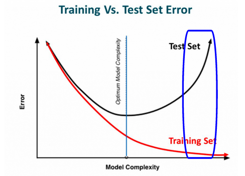
Since the validation accuracy is way less than the training accuracy, we can infer that the model is overfitting. The below illustration will give you a better understanding of what overfitting is:
The portion marked in blue in the above image is the overfitting model since training error is very less and the test error is very high. The reason for overfitting is that the model is learning even the unnecessary information from the training data and hence it performs really well on the training set.
But when new data is introduced, it fails to perform. We can introduce dropout to the model’s architecture to overcome this problem of overfitting.
Using dropout, we randomly switch off some of the neurons of the neural network. Let’s say we add a dropout of 0.5 to a layer which originally had 20 neurons. So, 10 neurons out of these 20 will be removed and we end up with a less complex architecture.
Hence, the model will not learn complex patterns and we can avoid overfitting. If you wish to learn more about dropouts, feel free to go through this article. Let’s now add a dropout layer to our architecture and check its performance.
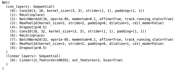
Model Architecture
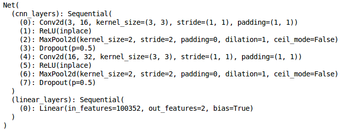
Here, I have added a dropout layer in each convolutional block. The default value is 0.5 which means that half of the neurons will be randomly switched off. This is a hyperparameter and you can pick any value between 0 and 1.
Next, we will define the parameters of the model like the loss function, optimizer, and learning rate.
Model Parameters
Here, you can see that the default value of p in dropout is 0.5. Finally, let’s train the model after adding the dropout layer:
Training the model
Let’s now check the training and validation accuracy using this trained model.
Checking model performance
Similarly, let’s check the validation accuracy:
Let’s compare this with the previous results:
| Training Accuracy | Validation Accuracy | |
| Without Dropout | 87.80 | 69.72 |
| With Dropout (p=0.5) | 73.56 | 70.29 |
The table above represents the accuracy without and with dropout. If you look at the training and validation accuracy of the model without dropout, they are not in sync. Training accuracy is too high whereas the validation accuracy is less. Hence, this was a possible case of overfitting.
When we introduced dropout, both the training and validation accuracies came in sync. Hence, if your model is overfitting, you can try to add dropout layers to it and reduce the complexity of the model.
The amount of dropout to be added is a hyperparameter and you can play around with that value. Let’s now look at another challenge.
Deep Learning Challenge #3: Model Underfitting
Deep learning models can underfit as well, as unlikely as it sounds.
Underfitting is when the model is not able to learn the patterns from the training data itself and hence the performance on the training set is low.
This might be due to multiple reasons, such as not enough data to train, architecture is too simple, the model is trained for less number of epochs, etc.
To overcome underfitting, you can try the below solutions:
- Increase the training data
- Make a complex model
- Increase the training epochs
For our problem, underfitting is not an issue and hence we will move forward to the next method for improving a deep learning model’s performance.
Deep Learning Challenge #4: Training Time is too High
There are cases when you might find that your neural network is taking a lot of time to converge. The main reason behind this is the change in the distribution of inputs to the layers of the neural network.
During the training process, the weights of each layer of the neural network change, and hence the activations also change. Now, these activations are the inputs for the next layer and hence the distribution changes with each successive iteration.
Due to this change in distribution, each layer has to adapt to the changing inputs – that’s why the training time increases.
To overcome this problem, we can apply batch normalization wherein we normalize the activations of hidden layers and try to make the same distribution.
You can read more about batch normalization in this article.
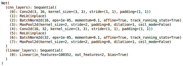
Let’s now add batchnorm layers to the architecture and check how it performs for the vehicle classification problem:
Defining model parameters
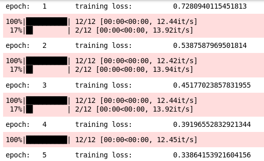
Let’s now train the model:
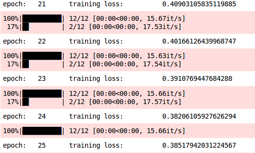
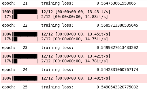
Clearly, the model is able to learn very quickly. We got a training loss of 0.3386 in the 5th epoch itself, whereas the training loss after the 25th epoch was 0.3851 (when we did not use batch normalization).
So, the introduction of batch normalization has definitely reduced the training time. Let’s check the performance on the training and validation sets:
Adding batch normalization reduced the training time but we have an issue here. Can you figure out what it is? The model is now overfitting since we got an accuracy of 91% on training and 63% on the validation set. Remember – we did not add the dropout layer in the latest model.
These are some of the tricks we can use to improve the performance of our deep learning model. Let’s now combine all the techniques that we have learned so far.
Case Study: Improving the Performance of the Vehicle Classification Model
We have seen how dropout and batch normalization help to reduce overfitting and quicken the training process. It’s finally time to combine all these techniques together and build a model.
Now, we will define the parameters for the model:
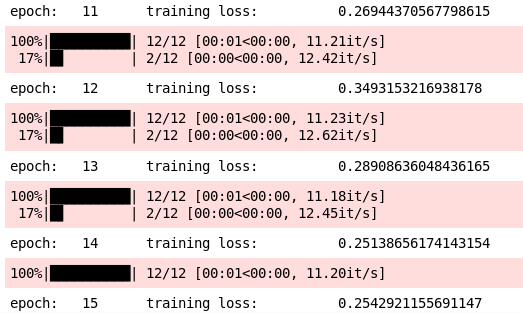
Finally, let’s train our model:
Next, let’s check the performance of the model:
The validation accuracy has clearly improved to 73%. Awesome!
End Notes
In this article, we looked at different challenges that we can face when using deep learning models like CNNs. We also learned the solutions to all these challenges and finally, we built a model using these solutions.
The accuracy of the model on the validation set improved after we added these techniques to the model. There is always scope for improvement and here are some of the things that you can try out:
- Tune the dropout rate
- Add or reduce the number of convolutional layers
- Add or reduce the number of dense layers
- Tune the number of neurons in hidden layers, etc.
Do share your results in the comments section below. And if you’re interested in dabbling in the world of deep learning, make sure you check out the below comprehensive course:


