What Does Gradient Descent Actually Mean

This article was published as a part of the Data Science Blogathon.

Introduction

In this article, we will see what actually gradient Descent is and why it became popular and why most of the algorithms in AI and ML follow this technique.

Before Starting this, what actually Gradient Descent means? , Sounds Odd Right!

Cauchy is the first person who proposed this idea of Gradient Descent in 1847

Well, the word gradient means an increase and decrease in a property or something! whereas Descent means the act of moving downwards. So, in total, the observation done while coming down and reaching to someplace and again moving up is termed as gradient Descent

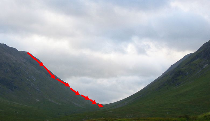
So, in normal terms as of in the picture, the sloppiness of the hill is high at the top, one single slip, and you are done! The sloppiness when you reach the bottom of the hill is minimal or close to or equal to zero, the same scenario works in Mathematics as well.

Let us find out how?

Mathematics of Gradient Descent

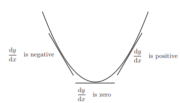
So, if you see here this is the same shape as the hill here. Let us assume that this is a curve that is of the form y=f(x). Here we know the slope at any point is the derivative of y with respect to x at that particular position, if you check this using any curve you will find out that slope while coming downwards decreases and equal to zero at the tip or at the minimal position and increases as we move up again

Keeping this in mind we will look at what happens to the x and y values at the minimal point,

If we observe carefully in the figure below, we have five points here at different positions!

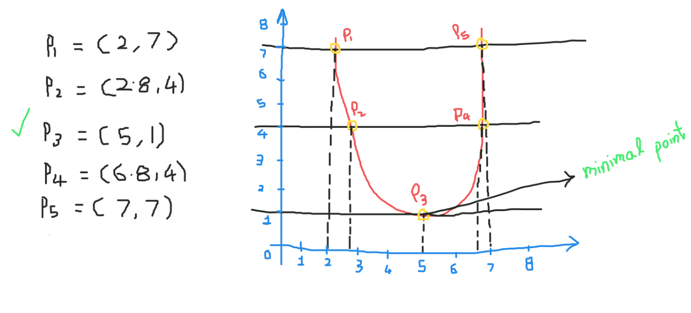
As we move downwards we are finding that our y value decreases w.r.t x value so out of all the points here we get comparatively minimal values at the bottom of the graph. So, our conclusion here is we always find the minimal (x,y) at the bottom of the graph. Now let us see how we can impart this in ML and DL and how to reach that minimal point without travelling the entire graph?

In any Algorithm, our main Motive is to minimize our loss that indicates that our model has performed well. For analyzing this we will use linear regression

 

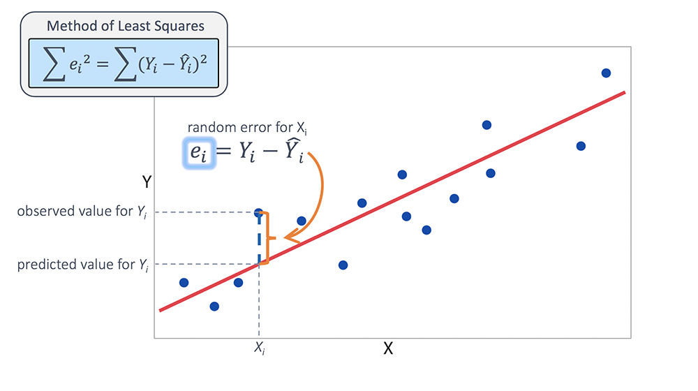
Since linear regression uses a line to predict the continuous output-

                  let the line be y = w * x + c

Here we need to find the w and c such that we get the best fit line that minimizes the error. So our aim is to find the optimal w and c values

We start w and c with some random values and we start updating these values w.r.t to the loss i.e we update these weights till our slope is equal to or close to zero.

We will take the loss function on the y-axis and w and c on the x-axis. Check the figure below-

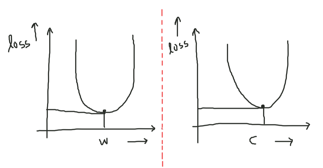
For reaching the minimal w value in the first graph follow these steps-

1. Start calculating the loss for the given set of x _values with the w and c.

2. Plot the point and now update the weight as-

                              w_new =w_old – learning_rate * slope at (w_old,loss)

Repeat these steps until you reach the minimal values!

* we are subtracting slope here because we want to move to the bottom of the hill or in the direction of steepest descent

* as we subtract our parameters gets updated and we will get a slope less than the previous one which is what we want to move to a point where the slope is equal to or close to zero

*we will talk about learning rate later!

The same applies to graph 2 also i.e loss vs c

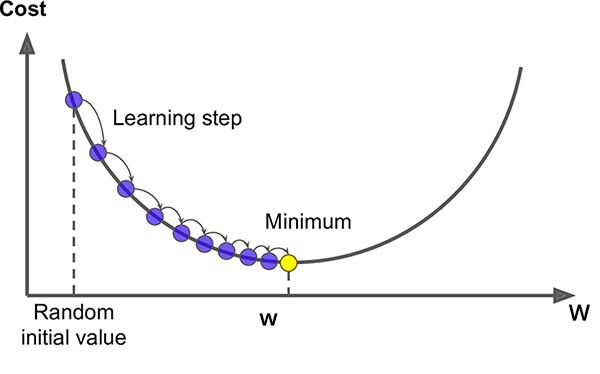
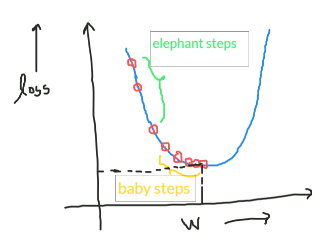
Now the question is why the learning rate is put in the equation? We cannot travel all the points present in between the starting point and the minimal point-

We need to skip some points-

• We can take elephant steps in the initial phase.
• But while moving near minima, we need to take baby steps, because we may cross over the minima and move to a point where slope increases.So in order to control the step size and the shift in the graph learning_rate was introduced. Even without the learning rate, we get the minimum value but what we are concerned about is that we want our algorithm to be faster !!!

  

  Here is a sample algorithm of how linear regression works using Gradient Descent. Here we use mean square error as a loss function-

  1. initializing model parameters with zeros m=0 , c=0
  2. initialize learning rate with any value in the range of (0,1) exclusive lr = 0.01

   

  You know the mean square error equation i.e-

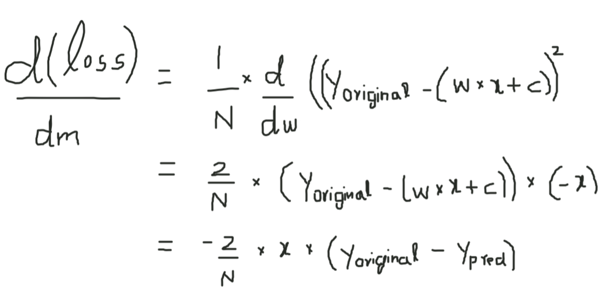
  Now substitute (w *x +c) in place of Ypred and differentiate w.r.t w

  

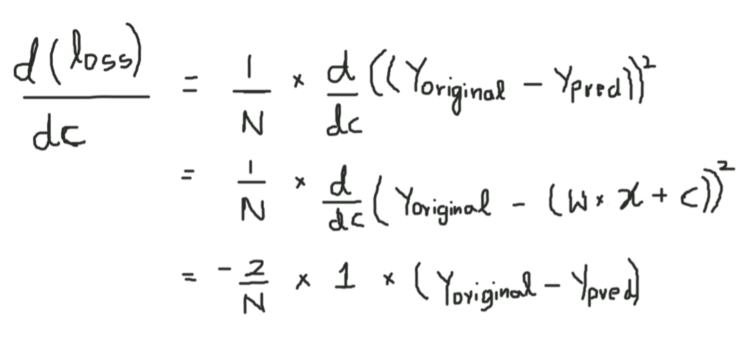
1. Here m in the L.H.S is noting but slope (w). Same with respect to c also-

   

    

2. Apply this for the given set of point in all the epochs

   for i in range(epochs):
             y_pred = w * x +c
             D_M = (-2/n) * sum(x * (y_original - y_pred))
             D_C = (-2/n) * sum(y_original - y_pred)
   
   
   

   * here sum function adds the gradient w.r.t all the points at one go!

Update the parameters for all iterations-
W = W – lr * D_M

C = C – lr * D_C

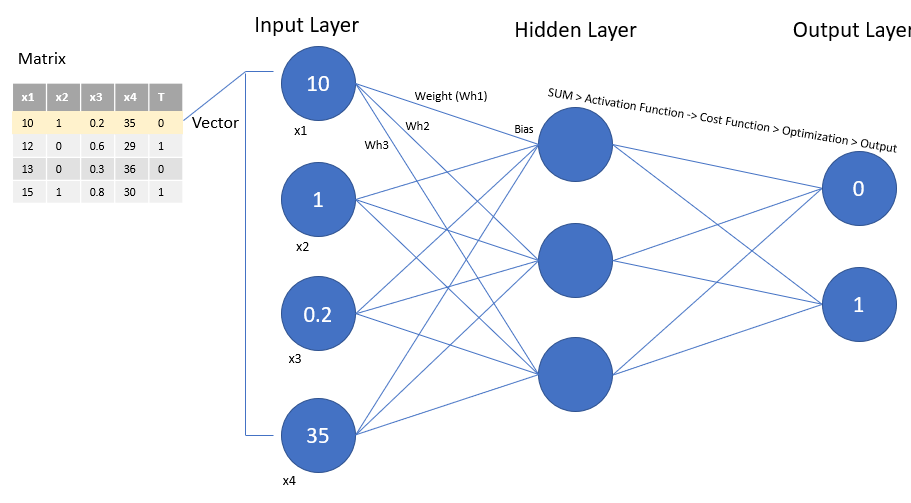
Gradient Descent is used in Deep Learning in Neural Networks also …

1. 

   Here we update the weights for each neuron so that we get the best classification with a minimal error we use gradient descent to update all the weights of every layer using backpropagation…

   W_i = W_i – learning_rate * derivative (Loss function w.r.t W_i)

Why it is popular?

1. Gradient descent is by far the most popular optimization strategy used in Machine Learning and Deep Learning at the moment.
2. It is used when training Data models, can be combined with every algorithm and is easy to understand and implement
3. Many statistical techniques and methods use GD to minimize and optimize their processes.

References

Phani Ratan

23 Dec 2020