Understand The Moment Generating Functions!

This article was published as a part of the Data Science Blogathon

Introduction

The probability distribution of a random variable can be expressed in many ways- Probability Density Functions (PDF) (or equivalently Probability Mass Functions, PMF for discrete variables), Cumulative Distribution Functions, Joint Probability distributions (for the relationship between the distributions), etc. The graphs of these functions can be described qualitatively and quantitatively.

Qualitative descriptions involve describing the characteristics of the graph without using numerical features. E.g., saying that the graph is broad, noisy, smooth, etc.

Quantitative descriptions, on the other hand, use numerical characteristics called moments. There are various such moments in statistics such as expected value, variance, skewness, kurtosis, median, mode, covariance, correlation, hypertailedness et al.

The massive realm of statistical sciences includes the detailed study of all of these moments of distributions. However, most of the statistical studies rely mainly on two of them- expected value and variance. Since the variance of a random variable can be obtained using different powers of the expected value, we’ll focus on the latter.

The expected value (or the mean) of a random variable is its weighted average. Mathematically, it is shown as:

This is often referred to as the first moment of a random variable X. Just as before,
we can define the 2^nd moment of a random variable [E(X²)]:

We follow a similar process to define the 3^rd, 4^th, 5^th, …, and eventually, the nth moment of a random variable [E(Xⁿ)] as follows:

Now suppose, we are given a normal distribution, and we are required to find its 1^st moment. Well, isn’t it simple? Just integrate x times the PDF over the entire range of the distribution. What about the 2^nd moment? Integrate x² times the PDF over the entire range of the distribution. And so on….

That’s a very tiring process, especially since it’s integration (or concurrently summation).

Is there an alternative method that can help us simplify things? Yes, here’s when Moment Generating Functions (MGFs) step in. Unlike the traditional method which relies on computing lengthy integrals, the method of MGFs eases the workload by relying on differentiation.

Besides, they have various other advantages, giving them a central role in statistical formulations. What are MGFs and how do they work? Let’s see!

What are Moment Generating Functions (MGFs)?

Think of moment generating functions as an alternative representation of the distribution of a random variable. Like PDFs & CDFs, if two random variables have the same MGFs, then their distributions are the same. Mathematically, an MGF of a random variable X is defined as follows:

A random variable X is said to have an MGF if:
1) M_x(t) exist for X.
2) The M_x(t) has a finite value for all t belonging to [-a, a], where a is any positive real number.

This may seem too much to digest at once. But we’ll understand it piece by piece.

First, what’s the t? Think of t as a constant whose value has got nothing to do with X. It allows the MGF to secretly encode the values of so many moments.

Second, how do we get the moments from the MGF? Just differentiate the MGF with respect to t, and let t=0! If you differentiate the MGF with respect to t once and substitute t=0, you’ll get the 1^st moment i.e., E(X). If you differentiate it once more, and now substitute t=0, you get the 2^nd moment i.e., E(X²). Likewise, if you differentiate the function n times and substitute t=0, you get the n^th moment i.e., E(Xⁿ).

The key point here is that the substitution t=0 must be done only at the end i.e., after differentiating the MGF the required
number of times. Mathematically,

Third, how does this work? We’ll understand the derivation of the above equation very soon. But before that, we need to understand the meaning of E(e^tX). It’s just equal to the expression obtained by replacing the X in the first equation of this article with e^tX:

Now, that we know the basics, we’ll prove that differentiating the MGF n times and substituting t=0 gives E(Xⁿ). We’ll use the Maclaurin series for e^x as follows:

We’ll now apply expectation on both sides and use the properties of expectation:

Differentiating both sides of the equation will give us:

At t=0, all the terms apart from E(X) get cancelled, giving:

This shows that the first derivative of the MGF at t=0 gives the 1^st moment of X. To prove that MGFs work for any nth moment in general, we differentiate E(e^tX) n times:

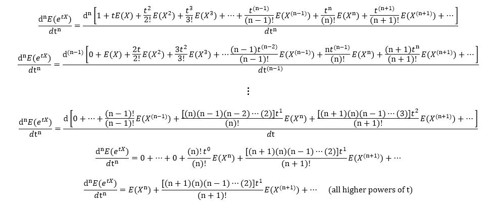
When we substitute t=0, all the higher powers of t cancel out, giving:

Some of us may have found it really hard to keep up with this derivation. Don’t worry! It’s enough if we just understand the essence i.e., how to use MGFs to find the different moments for different distributions. If you are really keen on understanding the derivation, read it once more and remember that:

1. The powers of X lesser than n (i.e., E(X¹), E(X²), …, E(X^(n-1))) are removed while differentiating the expression of e^tX n times (as they become constants).

2. The powers of X more than n (i.e., E(X⁽ⁿ⁺¹⁾), E(X⁽ⁿ⁺²⁾), …) are removed when we substitute t=0.

Thus, we’ll be left with E(Xⁿ), which proves our initial equation. Now we’ll understand a few basic properties of MGFs.

Basic Properties of Moment Gathering Functions

A) Moment Gathering Functions when a random variable undergoes a linear transformation:

Let X be a random variable whose MGF is known to be M_x(t). Suppose we have to find the MGF of a random variable Y, which is a linear transformation of X i.e., Y = αX + β. Then,

Since e^tβ is constant, we can take it out of the expectation, giving us the following equation:

Finally, we once again remember that t is simply a constant whose value has no correlation with X. Thus, we can consider the entire product ‘tα’ as the new constant giving us:

B)Moment Gathering Functions of a linear combination of several independent random variables:

Let X₁, X₂, …, X_n be independent random variables whose MGFs are known to be M_x1(t), M_x2(t), …, M_xn(t). Suppose we have to find the MGF of a random variable Y, which is a linear combination of X₁, X₂, …, X_n i.e., Y = α₁X₁ + α₂X₂ + … + α_nX_n + β. Following the same procedure as above, we get:

By the property of independence, we can separate the various terms:

More specifically, if Y is the sum of independent random variables, then the MGF of Y is the product of the MGFs of those random variable i.e., if Y = X₁ + X₂ + … + X_n

C) Case when the Moment Gathering Functions of two random variables are equal:

If X and Y are two random variables having the same MGF, thein their CDF is also the same i.e., their distributions are the same. Mathematically,

MGFs of some Special Distributions

Here, we’ll calculate the MGF & use it to derive the first moment of certain special distributions- Bernoulli, Binomial, Exponential, and Normal distribution.

A) Bernoulli Distribution

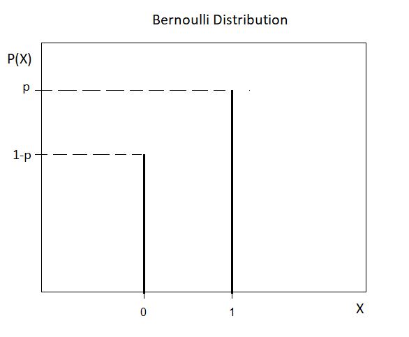
Bernoulli distribution is a discrete distribution having two possible outcomes- 1 (success) with a probability p & 0 (failure) with probability (1-p). The PMF of a Bernoulli distribution is defined as:

The following plot shows a Bernoulli distribution (with parameter p):

We’ll now derive its MGF as follows:

Calculating the first moment:

At t=0,

Thus, we have used MGF to obtain an expression for the first moment of a Bernoulli distribution.

B) Binomial Distribution

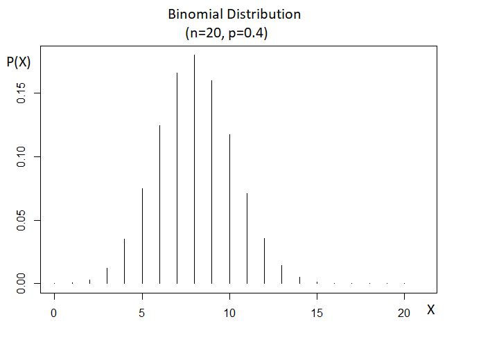
The binomial distribution is a sequence of several independent Bernoulli trials, with the probability of success p remaining constant for all the trials. In other words, the distribution of the sum of n i.i.d (independent & identically distributed) Bernoulli trials gives the binomial distribution:

The following plot shows a binomial distribution (with parameters p and n):

This time instead of using the PMF, we’ll use a shortcut- a property of MGFs. Recall that the MGF of the sum of several independent random variables is equal to the product of their MGFs:

We’ll use this property here. Let Y be the random variable having binomial distribution, and Xs be the random variables having Bernoulli distribution. We’ll derive the MGF of Y as follows (using the fact that they have identical distributions, and consequently the same MGF):

Calculating the first moment:

At t=0,

Thus, we have used MGF to obtain an expression for the first moment of Binomial distribution.

C) Exponential Distribution

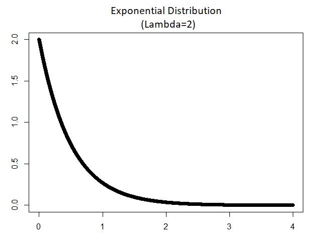
The PDF of an exponential distribution is defined as:

The following plot shows an exponential distribution (with parameter λ):

We’ll now derive its MGF as
follows:

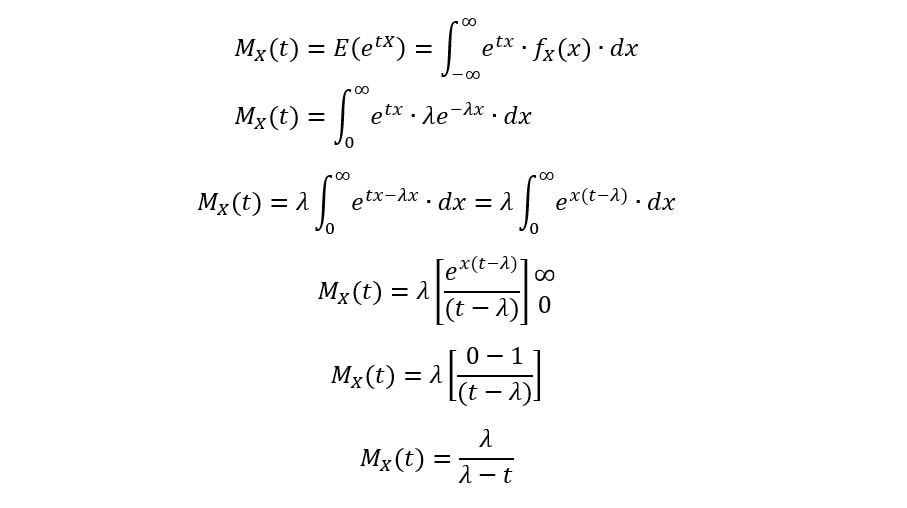
Calculating the first moment:

At t=0,

Thus, we have used MGF to obtain an expression for the first moment of an Exponential distribution.

D) Normal Distribution

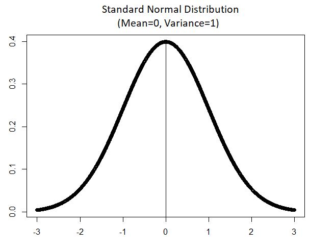
For the normal distribution, we’ll first discuss the case of standard normal, and then any normal distribution in general. A standard normal distribution has the mean equal to 0 and the variance equal to 1.

The PDF of a standard normal distribution is defined as:

The following plot shows an exponential distribution (with parameters µ and σ):

We’ll now derive its MGF as follows:

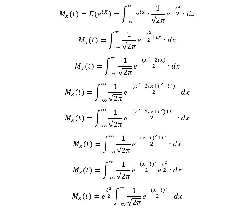
The integral corresponds to the PDF of a normal distribution with mean ‘t’, and variance 1. Thus, over the entire range of real interval, it integrates to 1 giving:

Now suppose we want to derive the MGF for any normal distribution in general with mean µ and variance σ^2. The PDF of such a distribution is shown as:

However, instead of integrating the entire expression again, we can use one of the properties of MGFs. A random variable Y having a normal distribution with mean µ and variance σ² can be related to a random variable X,
having standard normal distribution as follows:

Using the property of linear transformation of a random variable,

Thus, after a long derivation, we’ve obtained the MGF of any normal distribution in general. Calculating the first moment:

At t=0,

Thus, we have used MGF to obtain an expression for the first moment of a Normal distribution.

Conclusion

The concept of Moment Generating Functions has been thoroughly discussed in this article. The study of MGFs and their properties are very deep.

There are other concepts such as Jensen’s inequality, Chernoff bound, characteristic functions, etc.- all related to MGFs, which may be necessary for a statistician to know, but not so relevant for our study.

The media shown in this article are not owned by Analytics Vidhya and is used at the Author’s discretion.

FAQs