This article was published as a part of the Data Science Blogathon.
Overview
- Finishing in the top 10% in Machine Learning Hackathons is a simple process if you follow your intuitions, keep learning continuously, and experiment with great consistency
-
From a beginner in Hackathons a few months back, I have recently become a Kaggle Expert and one of the TOP 5 Contributors of Analytics Vidhya’s JanataHack Hackathon Series
-
I am here to share my knowledge and guide beginners to start their Hackathon journey
- This article assumes a basic understanding of terms like Machine Learning, Hackathons, Table Data, Classification, and Regression
Start your Data Science Hackathon Journey Today
Let’s Start with my Hackathon Journey. I have always wondered how to participate and ace data science hackathons but it was only when the country went into lockdown that I started exploring this.
I came across a wonderful Datacamp course called “Winning a Kaggle Competition in Python” to kick start my Hackathon journey. This 4 Hour course gave me an understanding of Hackathons and how to approach them. When we learn some new skill we have to test our skills in new platforms to apply our learnings.
While I was thinking of which platform to test my acquired knowledge, all of a sudden I got a notification from Analytics Vidhya (AV) for a Hackathon and the use cases were relatable to Data Science and Machine Learning use cases at work.
Without a second thought, I logged into AV, went to the hackathon section and selected Active Hackathons but there were too many to choose from! I was eager to start with a basic and easy to understand Problem as a beginner in Hackathons.
The HR Analytics problem really caught my eye and I was quite excited to start my first Hackathon. It’s an interesting Binary Classification problem – meaning the Target we are going to predict will have only 2 Categories – Yes ( Promoted ) or No ( Not Promoted).
Let’s Deep Dive into the HR Analytics Problem and get our hands dirty
Link to HR Analytics Hackathon!
Our client is a large MNC and they have 9 broad verticals across the organization. One of the problems the client is facing is around identifying the right people for promotion (only for the manager position and below) and prepare them in time. Currently the process, they are following is:
- They first identify a set of employees based on recommendations/past performance
- Selected employees go through the separate training and evaluation program for each vertical. These programs are based on the required skill of each vertical
- At the end of the program, based on various factors such as training performance, KPI completion (only employees with KPIs completed greater than 60% are considered), etc., the employee gets a promotion
For the above mentioned process, the final promotions are only announced after the evaluation and this leads to delay in transition to their new roles. Hence, the company needs our help in identifying the eligible candidates at a particular checkpoint so that they can expedite the entire promotion cycle.
Sharing my Data Science Hackathon Approach – How I reached 4th Rank among 3000+ Data Lovers
Let me help you kick start your Hackathon Journey right away with a 10 Step Process that can be repeated, optimized, and improved over time. Even though there are a few other steps in addition to these 10 Steps, this will be a great foundation to help you get started quickly and put you to practice.
Rest assured, you will be in a good position to tackle any Hackathons (with table data) with a few weeks of practice. Hope you are enthusiastic, curious to learn more, and excited to start this amazing Data Science journey with Hackathons!
10 Easy Steps to Learn, Practice and Top in Data Science Hackathons
- Understand the Problem Statement and Import the Packages and Datasets
- Perform EDA (Exploratory Data Analysis) – Understanding the Datasets. Explore Train and Test Data and get to know what each Column / Feature denotes. Check for Imbalance of Target Column in Datasets
- Check for Duplicate Rows from Train Data
- Fill/Impute Missing Values – Continuous – Mean/Median/Any Specific Value | Categorical – Others/ForwardFill/BackFill
- Feature Engineering – Feature Selection – Selection of Most Important Existing Features | Feature Creation or Binning – Creation of New Feature(s) from the Existing Feature(s)
- Split Train Data into Features(Independent Variables) | Target(Dependent Variable)
- Data Encoding – Label Encoding, One-Hot Encoding | Data Scaling – MinMaxScaler, StandardScaler, RobustScaler
- Create Baseline Machine Learning Model for the Binary Classification problem
- Ensemble with Voting Classifier to Improve the Evaluation Metric “F1-Score” and Predict Target “is_promoted”
- Result Submission, Check Leaderboard, and Improve “F1-Score”
1. Understand the Problem Statement and Import Packages and Datasets
Dataset Description
| Variable | Definition |
| employee_id | Unique ID for employee |
| department | Department of employee |
| region | Region of employment (unordered) |
| education | Education Level |
| gender | Gender of Employee |
| recruitment_channel | Channel of recruitment for employee |
| no_of_trainings | no of other trainings completed in previous year on soft skills, technical skills etc. |
| age | Age of Employee |
| previous_year_rating | Employee Rating for the previous year |
| length_of_service | Length of service in years |
| KPIs_met >80% | if Percent of KPIs(Key performance Indicators) >80% then 1 else 0 |
| awards_won? | if awards won during previous year then 1 else 0 |
| avg_training_score | Average score in current training evaluations |
| is_promoted | (Target) Recommended for promotion |
We are given multiple attributes based on an Employee’s past and current performance along with demographics. Now, our task is to predict whether a potential employee at a checkpoint in the test set will be promoted or not after the evaluation process.
Evaluation Metric used to Check Machine Learning Models Performance Differs in All Hackathons
- F1 score is the evaluation metric for this Hackathon. It is the harmonic mean of Precision and Recall:
F1 Score = 2* ( (precision*recall) / (precision+recall) )
- Precision is the number of correctly identified positive results divided by the number of all positive results, including those not identified correctly
- Recall is the number of correctly identified positive results divided by the number of all samples that should have been identified as positive
- F1 score provides a better measure of the incorrectly classified ones, than Accuracy metric since F1 score penalizes the extreme values
- HR Analytics Train Data consists of 54,808 examples, and the Test Data consists of 23,490 examples. Huge Imbalance in Data – only 8.5% (4668 out of total 54,808) of Employees were recommended for promotion based on Train data.
Let us start by Importing the required Python Packages
# Warning Libraries
warnings.filterwarnings("ignore")
# Scientific and Data Manipulation Libraries
import pandas as pd
import numpy as np
import math
import gc
import os
# Data Preprocessing, Machine Learning and Metrics Libraries
from sklearn.preprocessing            import LabelEncoder, OneHotEncoder
from sklearn.preprocessing            import StandardScaler, MinMaxScaler, RobustScaler, MaxAbsScaler
from sklearn.ensemble                 import VotingClassifier
from sklearn.metrics                  import f1_score
# Boosting Algorithms
from xgboost                          import XGBClassifier
from catboost                         import CatBoostClassifier
from lightgbm                         import LGBMClassifier
# Data Visualization Libraries
import matplotlib.pyplot as plt
import seaborn as sns
import plotly.io as pio
import plotly.graph_objects as go
import plotly.express as px
1. Warning Libraries – Used to ignore any warnings in libraries
2. Scientific and Data Manipulation – Used to manipulate Numeric data using Numpy and Table data using Pandas
3. Data Preprocessing, Machine Learning, and Metrics Libraries – Used to pre-process the data by encoding, scaling, ensembling, and measure the date using evaluating metrics like F1 Score
4. Boosting Algorithms – XGBoost, CatBoost, and LightGBM Tree-based Classifier Models are used for Binary as well as Multi-Class classification
5. Data Visualization Libraries – Matplotlib, Seaborn, and Plotly are used for visualization of the single or multiple variables
2. Perform EDA (Exploratory Data Analysis) – Understanding the Datasets
# Looks at the first 5 rows of the Train and Test data
train = pd.read_csv('1. Data/train.csv')
test = pd.read_csv('1. Data/test.csv')
# Looks at the first 5 rows of the Train and Test data
display('Train Head :',train.head())
display('Test Head :',test.head())
# Displays Information of Columns of Train and Test data
train.info()
test.info()
# Displaya Descriptive Statistics of Train and Test data
display('Train Description :',train.describe())
display('Test  Description :',test.describe())
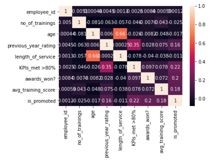
# Displays Correlation between Features through HeatMap - Ligther Color means Higher Correlation
sns.heatmap(train.corr(), annot = True);
Reading the Data Files in CSV Format – Pandas read_csv method is used to read the csv file and convert into a Table like Data structure called a DataFrame. So 2 DataFrames are created for Train and Test.
Apply Head on Data – Used to view the Top 5 rows to get an overview of the data.
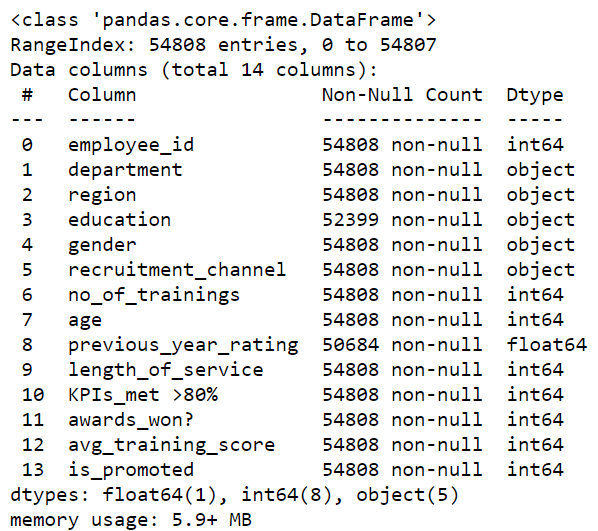
Apply Info on Data – Used to display information on Columns, Data Types and Memory usage of the DataFrames.
Apply Describe on Data – Used to display the Descriptive statistics like Count, Unique, Mean, Min, Max .etc on Numerical Columns.
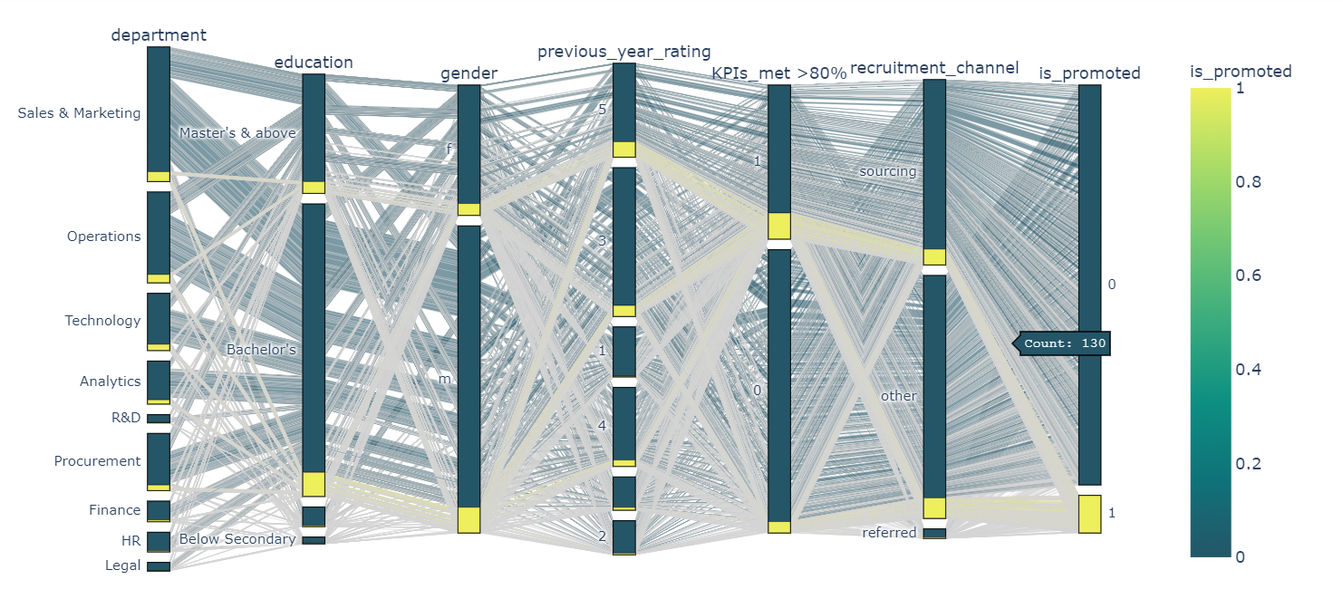
Data Visualization Libraries – Matplotlib, Seaborn, and Plotly are used for visualization of the single or multiple variables.
3. Check for Duplicate Rows from Train Data
# Removes Data Duplicates while Retaining the First one
def remove_duplicate(data):
    data.drop_duplicates(keep="first", inplace=True)
    return "Checked Duplicates"

# Removes Duplicates from train data
remove_duplicate(train)
Checking the Train Data for Duplicates – Removes the duplicate rows by keeping the first row. No duplicates were found in Train data.
4. Fill/Impute Missing Values – Continuous – Mean/Median/Zero(Specific Value) | Categorical – Forward/BackFill/Others
# Fills Missing Values in Train and Test :
train[ "previous_year_rating"} = train["previous_year_rating"}.fillna(0)
test["previous_year_rating"} = test["previous_year_rating"}.fillna(0)
# Creates a New Column to see if missing previous_year_rating and length_of_service = 1 Year are related
train['Fresher'} = train['previous_year_rating'}.apply(lambda x: 'Fresher' if x ==0 else 'Experienced')
display( train[["previous_year_rating","length_of_service",'Fresher'}}[train['Fresher'} =='Fresher'} )
train["education"} = train["education"}.ffill(axis = 0)
train["education"} = train["education"}.bfill(axis = 0)
test["education"} = test["education"}.ffill(axis = 0)
test["education"} = test["education"}.bfill(axis = 0)
display("Train : ", train.info())
display("Test: ", test.info())
There are Missing Values in 2 Columns “previous_year_rating” and “education”.
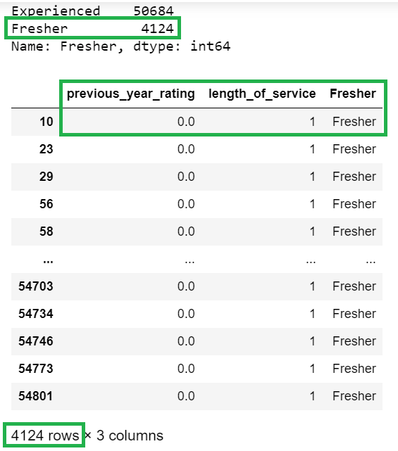
What is the Intuition that went on to filling the Column “previous_year_rating” using Zero – Let us think of, Why is the Data Missing in Column “previous_year_rating” in the first place?
- Upon closer look, data was not entered because those employees were Freshers (i.e) length_of_service is 1 Year
- No data would have been there in the data source itself for these employees. Logically we are filling missing values with “0” because Freshers with less than or equal to 1 Year of Experience may not have previous_year_rating at all
Filling Missing Values in Data – Filling missing value with Mode (Most frequently occurring value ) and introducing a New Category “Others” are the most commonly used techniques that didn’t work on the Column “education” as F1-Score reduced.
Apply ffill on Data – Used to forward fill that fills the current missing value with Previous Row value. If the previous row value is NaN (Not a Number) it moves to the next row without filling.
Apply bfill on Data – Used to Backward fill that fills the current missing value with Next Row Value. If the next row value is NaN (Not a Number) it moves to the next row without filling.
Since Ffill and Bfill worked well, we can assume that while Collecting data, relevant data of relevant employees with the same educational background were collected close to one another in a sequential manner.
5. Feature Engineering
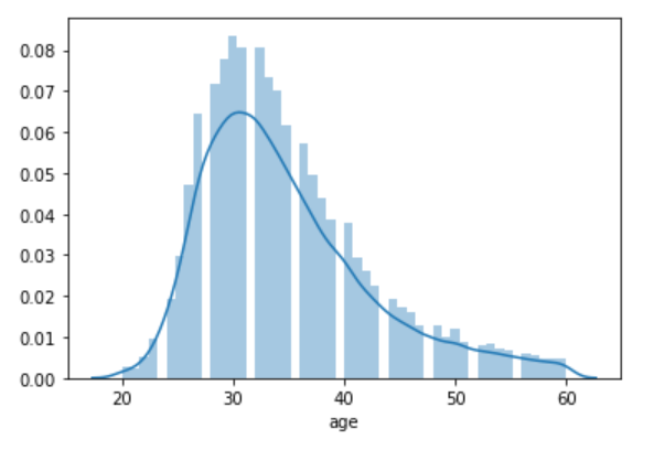
# Based on Age Distribution - Most of the Employees are in range 20-40 who will be also waiting for a Promotion
# so we have created 2 Bins 20-29, 29-39 and remaining 1 Bin for 39-49.
# displot -> plot a univariate(Single Feature) distribution of observations.
sns.distplot(train['age'})
train['age'} = pd.cut( x=train['age'}, bins=[20, 29, 39, 49}, labels=['20', '30', '40'} )
test['age'}  = pd.cut( x=test['age'}, bins=[20, 29, 39, 49},  labels=['20', '30', '40'} )
Based on Age Distribution – Most of the employees are in the range 20-40 who will be waiting for a promotion, so we have created 2 bins 20-29, 29-39, and the remaining 1 bin for 39-49.
6. Split Train Data into Features(Independent) & Target(Dependent)
# Split train into X_train (Features) and y_train (Target) :
X_train = train.drop('is_promoted',axis=1)
y_train = train['is_promoted'}
y_train = y_train.to_frame()
X_test = test
Split Train Data into Features and Target –Drop the Target column from the DataFrame to get the other features or independent variables.
7.1 Data Encoding: Label Encoding, OneHot Encoding
def data_encoding( encoding_strategy , encoding_data , encoding_columns ):
    if encoding_strategy == "LabelEncoding":
        print("IF LabelEncoding")
        Encoder = LabelEncoder()
        for column in encoding_columns :
            print("column",column )
            encoding_data[ column } = Encoder.fit_transform(tuple(encoding_data[ column }))
    elif encoding_strategy == "OneHotEncoding":
        print("ELIF OneHotEncoding")
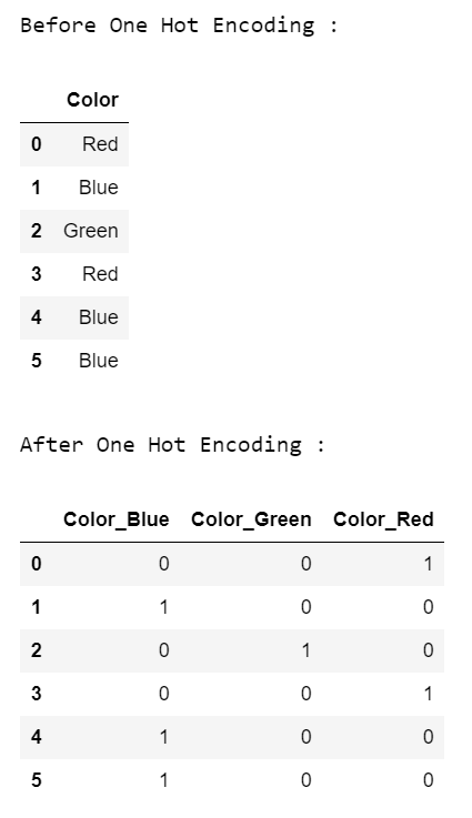
        encoding_data = pd.get_dummies(encoding_data)
    dtypes_list =['float64','float32','int64','int32'}
    encoding_data.astype( dtypes_list[0} ).dtypes
    return encoding_data
encoding_columns  = [ "region", "age","department", "education", "gender", "recruitment_channel" }
encoding_strategy = [ "LabelEncoding", "OneHotEncoding"}
X_train_encode = data_encoding( encoding_strategy[1} , X_train , encoding_columns )
X_test_encode =  data_encoding( encoding_strategy[1} , X_test  , encoding_columns )
# Display Encoded Train and Test Features :
display(X_train_encode.head())
display(X_test_encode.head())
One Hot Encoding will be applied only to Object or Categorical Columns . It is most common to one-hot encode these object columns. Pandas offers a convenient function called get_dummies to get one-hot encodings. Many machine learning algorithms cannot operate on label or categorical data directly. This means that categorical data must be converted to a numerical form. In One Hot Encoding the integer encoded variable is removed and a New Binary variable is added for each Unique label or category value – Jason Brownlee
def data_scaling( scaling_strategy , scaling_data , scaling_columns ):
    if    scaling_strategy =="RobustScaler" :
        scaling_data[scaling_columns} = RobustScaler().fit_transform(scaling_data[scaling_columns})
    elif  scaling_strategy =="StandardScaler" :
        scaling_data[scaling_columns} = StandardScaler().fit_transform(scaling_data[scaling_columns})
    elif  scaling_strategy =="MinMaxScaler" :
        scaling_data[scaling_columns} = MinMaxScaler().fit_transform(scaling_data[scaling_columns})
    elif  scaling_strategy =="MaxAbsScaler" :
        scaling_data[scaling_columns} = MaxAbsScaler().fit_transform(scaling_data[scaling_columns})
    else :  # If any other scaling send by mistake still perform Robust Scalar
        scaling_data[scaling_columns} = RobustScaler().fit_transform(scaling_data[scaling_columns})
    return scaling_data
# RobustScaler is better in handling Outliers :
scaling_strategy = ["RobustScaler", "StandardScaler","MinMaxScaler","MaxAbsScaler"}
X_train_scale = data_scaling( scaling_strategy[0} , X_train_encode , X_train_encode.columns )
X_test_scale  = data_scaling( scaling_strategy [0} , X_test_encode  , X_test_encode.columns )
# Display Scaled Train and Test Features :
display(X_train_scale.head())
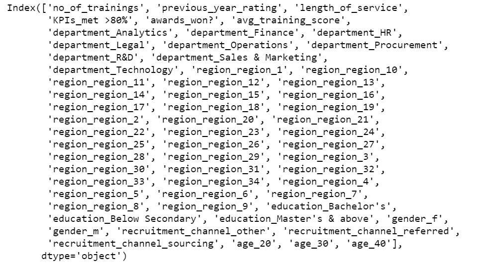
display(X_train_scale.columns)
display(X_train_scale.head())
Standardization of a dataset is a common requirement for many machine learning estimators. Typically this is done by removing the mean and scaling to unit variance like StandardScaler.
Outliers can often influence the sample mean and variance. RobustScaler which uses the median and the interquartile range often gives better results as it gave for this dataset.
8. Create Baseline Machine Learning Model for Binary Classification Problem
# Baseline Model Without Hyperparameters :
Classifiers = {'0.XGBoost' : XGBClassifier(),
               '1.CatBoost' : CatBoostClassifier(),
               '2.LightGBM' : LGBMClassifier()
 }
# Fine Tuned Model With-Hyperparameters :
Classifiers = {'0.XGBoost' : XGBClassifier(learning_rate =0.1,
                                           n_estimators=494,
                                           max_depth=5,
                                           subsample = 0.70,
                                           verbosity = 0,
                                           scale_pos_weight = 2.5,
                                           updater ="grow_histmaker",
                                           base_score  = 0.2),
               '1.CatBoost' : CatBoostClassifier(learning_rate=0.15,
                                                 n_estimators=494,
                                                 subsample=0.085,
                                                 max_depth=5,
                                                 scale_pos_weight=2.5),
               '2.LightGBM' : LGBMClassifier(subsample_freq = 2,
                                             objective ="binary",
                                             importance_type = "gain",
                                             verbosity = -1,
                                             max_bin = 60,
                                             num_leaves = 300,
                                             boosting_type = 'dart',
                                             learning_rate=0.15,
                                             n_estimators=494,
                                             max_depth=5,
                                             scale_pos_weight=2.5)
 }
Here we have reached Modelling. The most Interesting and Exciting part of the whole Hackathon to me is Modelling but we need to understand it is only 5-10 % of the Data Science Lifecycle.
Top winners of Kaggle and Analytics Vidhya Data Science Hackathons mostly use Gradient Boosting Machines (GBM).
1. LightGBM and its Hyperparameters
1. What is LightGBM?
- LightGBM is a gradient boosting framework that uses tree based learning algorithm.
2. How does it differ from other tree-based algorithms?
- LightGBM grows trees vertically while other algorithms grow trees horizontally meaning that this algorithm grows tree leaf-wise (row by row) while other algorithms grow level-wise.
3. How does it Work?
- It will choose the leaf with max delta loss to grow. When growing the same leaf, Leaf-wise algorithm can reduce more loss (in that it chooses the leaf it believes will yield the largest decrease in loss) than a level-wise algorithm but is prone to over-fitting.
LightGBM is faster than XGBoost and it is 20 times faster with the same performance is what LightGBM’s creators claim.
Key LightGBM Hyperparameter(s) Tuned in this Hackathon:
1. scale_pos_weight=2.5
scale_pos_weight, default = 1.0, type = double, constraints: scale_pos_weight > 0.0
- used only in
binaryandmulticlassovaapplications - weight of labels with positive class
- Note: while enabling this should increase the overall performance metric of your model, it will also result in poor estimates of the individual class probabilities
- Note: this parameter cannot be used at the same time with
is_unbalance, choose only one of them -
Only 8.5% (4668 out of total 54,808) of Employees were recommended for promotion based on Train data.
- scale_pos_weight = 54,808 / 4668 but since we have a huge imbalance we need to take the Square root of √ (54,808 / 4668) = 3.42. We can start from 3.42 to 1 unit below and above so we can cover a range of values from 2.42 to 4.42. We can finalize with 2.5 as it gave good results.
2. boosting_type = ‘dart’
boosting_type default = gbdt, type = enum, options: gbdt, rf, dart, goss, aliases: boosting_type, boost
gbdt, traditional Gradient Boosting Decision Tree, aliases:gbrt( Stable and Reliable )rf, Random Forest, aliases:random_forestdart, Dropouts meet Multiple Additive Regression Trees ( Used ‘dart’ for Better Accuracy as suggested in Parameter Tuning Guide for LGBM for this Hackathon and worked so well though ‘dart’ is slower than default ‘gbdt’ )goss, Gradient-based One-Side Sampling- Note: internally, LightGBM uses
gbdtmode for the first1 / learning_rateiterations
- Note: internally, LightGBM uses
3. n_estimators=494
As per the Parameter Tuning Guide for LGBM for Better Accuracyused small learning_rate with large num_iterations.
num_iterations , default = 100, type = int, aliases: num_iteration, n_iter, num_tree, num_trees, num_round, num_rounds, num_boost_round, n_estimators, constraints: num_iterations >= 0
- number of boosting iterations
- Note: internally, LightGBM constructs
num_class * num_iterationstrees for multi-class classification problems
4. learning_rate=0.15
learning_rate , default = 0.1, type = double, aliases: shrinkage_rate, eta, constraints: learning_rate > 0.0
- shrinkage rate
- in
dart, it also affects on normalization weights of dropped trees.
5. max_depth=5
max_depth , default = -1, type = int
-
To deal with over-fitting restrict the max depth of the tree model when data is small. The tree still grows leaf-wise
-
< = 0 means no restriction
2. XGBoost and its Hyperparameters
1. What is XGBoost?
- XGBoost (eXtreme Gradient Boosting) is an implementation of gradient boosted decision trees designed for speed and performance.
- XGBoost is an algorithm that has recently been dominating machine learning Kaggle competitions for tabular data.
2. How it differs from other tree-based algorithms?
- XGBoost makes use of a greedy algorithm (in conjunction with many other features).
3. How does it Work?
- XGboost has an implementation that can produce high-performing model trained on large amounts of data in a very short amount of time.
XGBoost wins you Hackathons most of the times, is what Kaggle and Analytics Vidhya Hackathon Winners claim!
Key XGBoost Hyperparameter(s) Tuned in this Hackathon
1. subsample = 0.70
subsample default=1
- Subsample ratio of the training instances. Setting it to 0.5 means that XGBoost would randomly sample half of the training data prior to growing trees. and this will prevent overfitting. Subsampling will occur once in every boosting iteration.
- range: (0,1}
2. updater =”grow_histmaker”
updater default= grow_colmaker,prune
- A comma-separated string defining the sequence of tree updaters to run, providing a modular way to construct and to modify the trees. This is an advanced parameter that is usually set automatically, depending on some other parameters. However, it could be also set explicitly by a user. The following updaters exist:
grow_colmaker: non-distributed column-based construction of trees.grow_histmaker: distributed tree construction with row-based data splitting based on the global proposal of histogram counting.grow_local_histmaker: based on local histogram counting.grow_quantile_histmaker: Grow tree using a quantized histogram.grow_gpu_hist: Grow tree with GPU.sync: synchronizes trees in all distributed nodes.refresh: refreshes tree’s statistics and/or leaf values based on the current data. Note that no random subsampling of data rows is performed.prune: prunes the splits
3. base_score=0.2
base_score default=0.5
- The initial prediction score of all instances, global bias
- For a sufficient number of iterations, changing this value will not have too much effect.
3. CatBoost and its Hyperparameters :
1. What is CatBoost?
- CatBoost is a high-performance open source library for gradient boosting on decision trees.
- CatBoost is derived from two words Category and Boosting.
2. Advantages of CatBoost over the other 2 Models?
- Very High performance with little parameter tuning as you can see the above code compared to other 2
- Handling of Categorical variables automatically with a Special Hyperparameter “cat_features“.
- Fast and scalable GPU version with CatBoost.
- In my experiments with Hackathons and Real world data, Catboost is the Most Robust Algorithm among the 3, check the score below for this Hackathon too.
3. How does it work better?
- CatBoost can handle categorical variables through 6 different methods of quantization, a statistical method that finds the best mapping of classes to numerical quantities for the model.
- CatBoost algorithm is built in such a way very less tuning is necessary, this leads to less overfitting and better generalization overall.
Key CatBoost Hyperparameter(s) Tuned in this Hackathon :
1. subsample = 0.085
- Also known as “sample rate for bagging” can be used if one of the following bootstrap types is selected :
- Poisson
- Bernoulli
- MVS
- The default value depends on the dataset size and the bootstrap type:
- Datasets with less than 100 objects, default =
1 - Datasets with 100 objects or more and :
- Poisson, Bernoulli — default =
0.66 - MVS — default =
0.80 - By default, the method for sampling the weights of objects is set to “Bayesian”. The training is performed faster if the “Bernoulli” method is set and the value for the sample rate for bagging is smaller than 1.
9. Ensemble with Voting Classifier to Improve the – “F1-Score” and Predict Target “is_promoted”
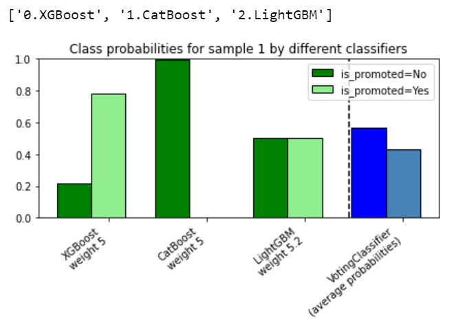
voting_model = VotingClassifier(estimators=[

('XGBoost_Best', list(Classifiers.values{})[0}),
('CatBoost_Best', list(Classifiers.values{})[1}),
('LightGBM_Best', list(Classifiers.values{})[2}),
},
voting='soft',weights=[5,5,5.2})
voting_model.fit(X_train_scale,y_train)
predictions_of_voting = voting_model.predict_proba( X_test_scale )[::,1}
Max Voting using Voting Classifier: Max voting method is generally used for classification problems. In this technique, multiple models are used to make predictions for each data point. The predictions by each model are considered as a ‘vote’. The predictions which we get from the majority of the models are used as the final prediction.
Example: If we ask 5 of our Readers to rate this Article (out of 5): We’ll assume three of them rated it as 5 while two of them gave it a 4. Since the majority gave a rating of 5, the final rating of this article will be taken as 5 out of 5. You can consider this similar to taking the mode of all the predictions.
Voting Classifier supports two types of voting:
Hard Voting : In hard voting, the predicted output class is a class with the highest majority of votes i.e the class which had the highest probability of being predicted by each of the classifiers. Suppose 5 classifiers predicted the output class(A,B,A, A, B), so here the majority predicted A as output. Hence A will be the final prediction.
Soft Voting : In soft voting, the output class is the prediction based on the average of probability given to that class. Suppose given some input to three models, the prediction probability for class A = (0.30, 0.47, 0.53) and B = (0.20, 0.32, 0.40). So the average for class A is 0.4333 and B is 0.3067, the winner is clearly class A because it had the highest probability averaged by each classifier.
Note: We need to make sure to include a variety of models to feed a Voting Classifier to be sure that the error made by one might be resolved by the other.
10. Result Submission, Check Leaderboard & Improve “F1” Score
# Round off the Probability Results :
predictions = [int(round{value}) for value in predictions_of_voting}
# Create a Dataframe Table for Submission Purpose :
Result_Promoted = pd.DataFrame({'employee_id': test["employee_id"}, 'is_promoted' : predictions})
Result_Promoted.to_csv("result.csv",index=False)
Strategy and Experiments in HR Analytics Hackathon
Analytics Vidhya Solution Checker Feature: We can make ANY Number of Submissions to Check the Leaderboard Score. This Technique is called Leaderboard Probing as we have tuned our Models based on Leaderboard Score instead of an essential Local Cross-Validation Score (which we will see in detail in Part 2 of this Hackathon Series).
In Real-world scenarios, we need to build a strong Local Cross-Validation Strategy.
Experiment 1: We need to start experimenting with various Machine Learning Models starting from the below list:
- Decision Tree – Score: 0.3964
- Logistic Regression – Score: 0.3964
- Random Forest – Score: 0.4045
Experiment 2: Since all of the above 3 Models gives an F1 Score close to 40% in the Leaderboard and Top Ranks have close to 53-54% F1 Scores, we can try all the 3 Tree-Based Boosting Models as we have discussed above to get better scores and reach better overall ranks.
- XGBoost Baseline model without Hyperparameter Tuning – Score: 0.4816
- CatBoost Baseline model without Hyperparameter Tuning – Score: 0.4851 – ROBUST
- LightGBM Baseline model without Hyperparameter Tuning – Score: 0.4798
Now we have reached a range of 47-48 % F1-Score with all 3 Boosted models.
Experiment 3: Let us Tune these models to get the best out of all 3 because Target is highly imbalanced as scale_pos_weight = 2.5 helped the most to tackle the imbalance.
- XGBoost Fine-Tuned Model with Hyperparameter Tuning – Score: 0.5138
- CatBoost Fine-Tuned Model with Hyperparameter Tuning – Score: 0.5273 – ROBUST
- LightGBM Fine-Tuned Model with Hyperparameter Tuning – Score: 0.5196
After fine-tuning the hyperparameters, F1-Score reached >51% in all 3 models. Now we are close to the Top Ranks ha 53-54% F1 Scores. Now we have a chance as it is only a 2% difference in the Scores.
Experiment 4 : To get a good F1-Score and Reach Top Ranks, Let us try to Average 3 ML Model Predictions using Voting Classifier Technique with both HARD and SOFT Voting (with Weights) :
- HARD Voting Classifier – Score: 0.5298
- SOFT Voting Classifier – Score: 0.5337 – BEST with RANK 4 Position
We have finally reached the Top 4 Rank of the HR Analytics Hackathon. The journey has been a roller coaster ride with lots and lots of learnings and experiments with intuition, logic, and application of Data Science Concepts.
Always focus on the Problem and know how much impact our predictions will make and Build Stable and Robust Models that will run quick and can generalize on new unseen data over Winning the Hackathons. This change in focus will surely help a lot in Real-World Scenarios of Data Science. – Vetrivel_PS
We have tried to solve the problem of predicting the right employees for Promotion. If it is a Real-World setup, solving this problem will have a Huge Impact for both the Client’s Company for decision making and Deserving Candidates who can move up in their career – a WIN-WIN Situation!
Top Rank Solution Approaches that were shared – Check Leaderboard here – Rank 13, Rank 14, and Rank 28!
Special Mention – These Solutions were my motivations so that I could one day hope to equal or better these Ranks with a Simpler Solution!
End Notes for Part 1 – Series to be Continued!
Here we have a much simpler Rank 4 Solution using our 10 Step Beginners Approach.
Happy to take you all through My First Hackathon journey to reach a Top Rank. Thanks a lot for reading if you find this article helpful please share it with Data Science Beginners to get started with Hackathons and keep waiting for Part 2 of this Hackathon Series which will explain many more steps like Cross-Validation, Running Models in GPU, Blending and Stacking of multiple models.
Thanks again for reading and showing your support friends. 🙂


