Introduction
Natural Language Processing (NLP) needs no introduction in today’s world. It’s one of the most important fields of study and research, and has seen a phenomenal rise in interest in the last decade. The basics of NLP are widely known and easy to grasp. But things start to get tricky when the text data becomes huge and unstructured.
That’s where deep learning becomes so pivotal. Yes, I’m talking about deep learning for NLP tasks – a still relatively less trodden path. DL has proven its usefulness in computer vision tasks like image detection, classification and segmentation, but NLP applications like text generation and classification have long been considered fit for traditional ML techniques.

Source: Tryolabs
And deep learning has certainly made a very positive impact in NLP, as you’ll see in this article. We will focus on the concept of transfer learning and how we can leverage it in NLP to build incredibly accurate models using the popular fastai library. I will introduce you to the ULMFiT framework as well in the process.
Note- This article assumes basic familiarity with neural networks, deep learning and transfer learning. If you are new to deep learning, I would strongly recommend reading the following articles first:
- An Introductory Guide to Deep Learning and Neural Networks
- A Complete Guide on Getting Started with Deep Learning in Python
If you are a beginner in NLP, check out this video course with 7 real life projects.
Table of Contents
- The Advantage of Transfer Learning
- Pre-trained Models in NLP
- Overview of ULMFiT
- Understanding the Problem Statement
- System Setup: Google Colab
- Implementation in Python
- What’s Next?
The Advantage of Transfer Learning
I praised deep learning in the introduction, and deservedly so. However, everything comes at a price, and deep learning is no different. The biggest challenge in deep learning is the massive data requirements for training the models. It is difficult to find datasets of such huge sizes, and it is way too costly to prepare such datasets. It’s simply not possible for most organizations to come up with them.
Another obstacle is the high cost of GPUs needed to run advanced deep learning algorithms.
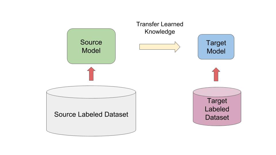
Thankfully, we can use pre-trained state-of-the-art deep learning models and tweak them to work for us. This is known as transfer learning. It is not as resource intensive as training a deep learning model from scratch and produces decent results even on small amounts of training data. This concept will be expanded upon later in the article when we implement our learning on quite a small dataset.
Pre-trained Models in NLP
Pre-trained models help data scientists start off on a new problem by providing an existing framework they can leverage. You don’t always have to build a model from scratch, especially when someone else has already put in their hard work and effort! And these pre-trained models have proven to be truly effective and useful in the field of computer vision (check out this article to see our pick of the top 10 pre-trained models in CV).
Their success is popularly attributed to the Imagenet dataset. It has over 14 million labeled images with over 1 million images also accompanying bounding boxes. This dataset was first published in 2009 and has since become one of the most sought-after image datasets ever. It led to several breakthroughs in deep learning research for computer vision, with transfer learning being one of them.
However, in NLP, transfer learning has not been as successful (as compared to computer vision, anyway). Of course we have pre-trained word embeddings like word2vec, GloVe, and fastText, but they are primarily used to initialize only the first layer of a neural network. The rest of the model still needs to be trained from scratch and it requires a huge number of examples to produce a good performance.
What do we really need in this case? Like the aforementioned computer vision models, we require a pre-trained model for NLP which can be fine-tuned and used on different text datasets. One of the contenders for pre-trained natural language models is the Universal Language Model Fine-tuning for Text Classification, or ULMFiT (Imagenet dataset [cs.CL]).
How does it work? How widespread are it’s applications? How can we make it work in Python? In the rest of this article, we will put ULMFiT to the test by solving a text classification problem and check how well it performs.
Overview of ULMFiT
Proposed by fast.ai’s Jeremy Howard and NUI Galway Insight Center’s Sebastian Ruder, ULMFiT is essentially a method to enable transfer learning for any NLP task and achieve great results. All this, without having to train models from scratch. That got your attention, didn’t it?
ULMFiT achieves state-of-the-art result using novel techniques like:
- Discriminative fine-tuning
- Slanted triangular learning rates, and
- Gradual unfreezing
This method involves fine-tuning a pre-trained language model (LM), trained on the Wikitext 103 dataset, to a new dataset in such a manner that it does not forget what it previously learned.
Language modeling ( covered in this course) can be considered a counterpart of Imagenet for NLP. It captures general properties of a language and courseprovides an enormous amount of data which can be fed to other downstream NLP tasks. That is why Language modeling has been chosen as the source task for ULMFiT.
I highly encourage you to go through the original ULMFiT paper to understand more about how it works, the way Jeremy and Sebastian went about deriving it, and parse through other interesting details.
Problem Statement
Alright, enough theoretical concepts – let’s get our hands dirty by implementing ULMFiT on a dataset and see what the hype is all about.
Our objective here is to fine-tune a pre-trained model and use it for text classification on a new dataset. We will implement ULMFiT in this process. The interesting thing here is that this new data is quite small in size (<1000 labeled instances). A neural network model trained from scratch would overfit on such a small dataset. Hence, I would like to see whether ULMFiT does a great job at this task as promised in the paper.
Dataset: We will use the 20 Newsgroup dataset available in sklearn.datasets. As the name suggests, it includes text documents from 20 different newsgroups.
System Setup: Google Colab
We will perform the python implementation on Google Colab instead of our local machines. If you have never worked on colab before, then consider this a bonus! Colab, or Google Colaboratory, is a free cloud service for running Python. One of the best things about it is that it provides GPUs and TPUs for free and hence, it is pretty handy for training deep learning models.
Some major benefits of Colab:
- Completely free of cost
- Comes with pretty decent hardware configuration
- Connected to your Google Drive
- Very well integrated with Github
- And many more features you’ll discover as you play around with it..
So, it doesn’t matter even if you have a system with pretty ordinary hardware specs – as long as you have a steady internet connection, you are good to go. The only other requirement is that you must have a Google account. Let’s get started!
Implementation in Python
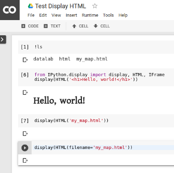
First, sign in to your Google account. Then select ‘NEW PYTHON 3 NOTEBOOK’. This notebook is similar to your typical Jupyter Notebook, so you won’t have much trouble working on it if you are familiar with the Jupyter environment. A Colab notebook looks something like the screenshot below:
Then go to Runtime, select Change runtime type, then select GPU as the hardware accelerator to utilise GPU for free.
Import Required Libraries
Most of the popular libraries like pandas, numpy, matplotlib, nltk, and keras, come preinstalled with Colab. However, 2 libraries, PyTorch and fastai v1 (which we need in this exercise), will need to be installed manually. So, let’s load them into our Colab environment:
!pip install torch_nightly -f https://download.pytorch.org/whl/nightly/cu92/torch_nightly.html
!pip install fastai
# import libraries
import fastai
from fastai import *
from fastai.text import *
import pandas as pd
import numpy as np
from functools import partial
import io
import os
Import the dataset which we downloaded earlier.
from sklearn.datasets import fetch_20newsgroups
dataset = fetch_20newsgroups(shuffle=True, random_state=1, remove=('headers', 'footers', 'quotes'))
documents = dataset.data
Let’s create a dataframe consisting of the text documents and their corresponding labels (newsgroup names).
df = pd.DataFrame({'label':dataset.target, 'text':dataset.data})
df.shape
(11314, 2)
We’ll convert this into a binary classification problem by selecting only 2 out of the 20 labels present in the dataset. We will select labels 1 and 10 which correspond to ‘comp.graphics’ and ‘rec.sport.hockey’, respectively.
df = df[df['label'].isin([1,10])]
df = df.reset_index(drop = True)
Let’s have a quick look at the target distribution.
df['label'].value_counts()
10    600
1     584
Name: label, dtype: int64
The distribution looks pretty even. Accuracy would be a good evaluation metric to use in this case.
Data Preprocessing
It’s always a good practice to feed clean data to your models, especially when the data comes in the form of unstructured text. Let’s clean our text by retaining only alphabets and removing everything else.
df['text'] = df['text'].str.replace("[^a-zA-Z]", " ")
Now, we will get rid of the stopwords from our text data. If you have never used stopwords before, then you will have to download them from the nltk package as I’ve shown below:
import nltk
nltk.download('stopwords')

from nltk.corpus import stopwords
stop_words = stopwords.words('english')
# tokenization
tokenized_doc = df['text'].apply(lambda x: x.split())

# remove stop-words
tokenized_doc = tokenized_doc.apply(lambda x: [item for item in x if item not in stop_words])

# de-tokenization
detokenized_doc = []
for i in range(len(df)):
    t = ' '.join(tokenized_doc[i])
    detokenized_doc.append(t)

df['text'] = detokenized_doc
Now let’s split our cleaned dataset into training and validation sets in a 60:40 ratio.
from sklearn.model_selection import train_test_split

# split data into training and validation set
df_trn, df_val = train_test_split(df, stratify = df['label'], test_size = 0.4, random_state = 12)
df_trn.shape, df_val.shape
((710, 2), (474, 2))
Perfect!
Before proceeding further, we’ll need to prepare our data for the language model and for the classification model separately. The good news? This can be done quite easily using the fastai library:
# Language model data
data_lm = TextLMDataBunch.from_df(train_df = df_trn, valid_df = df_val, path = "")

# Classifier model data
data_clas = TextClasDataBunch.from_df(path = "", train_df = df_trn, valid_df = df_val, vocab=data_lm.train_ds.vocab, bs=32)
Fine-Tuning the Pre-Trained Model and Making Predictions
We can use the data_lm object we created earlier to fine-tune a pre-trained language model. We can create a learner object, ‘learn’, that will directly create a model, download the pre-trained weights, and be ready for fine-tuning:
learn = language_model_learner(data_lm, pretrained_model=URLs.WT103, drop_mult=0.7)
The one cycle and cyclic momentum allows the model to be trained on higher learning rates and converge faster. The one cycle policy provides some form of regularisation. We won’t go into the depth of how this works as this article is about learning the implementation. However, if you wish to know more about one cycle policy, then feel free to refer to this excellent paper by Leslie Smith – “A disciplined approach to neural network hyper-parameters: Part 1 — learning rate, batch size, momentum, and weight decay”.
# train the learner object with learning rate = 1e-2
learn.fit_one_cycle(1, 1e-2)
Total time: 00:09
| epoch | train_loss | valid_loss | accuracy |
|---|---|---|---|
| 1 | 7.803613 | 6.306118 | 0.139369 |
We will save this encoder to use it for classification later.
learn.save_encoder('ft_enc')
Let’s now use the data_clas object we created earlier to build a classifier with our fine-tuned encoder.
learn = text_classifier_learner(data_clas, drop_mult=0.7)
learn.load_encoder('ft_enc')
We will again try to fit our model.
learn.fit_one_cycle(1, 1e-2)
Total time: 00:32
| epoch | train_loss | valid_loss | accuracy |
|---|---|---|---|
| 1 | 0.534962 | 0.377784 | 0.907173 |
Wow! We got a whopping increase in the accuracy and even the validation loss is far less than the training loss. It is a pretty outstanding performance on a small dataset. You can even get the predictions for the validation set out of the learner object by using the below code:
# get predictions
preds, targets = learn.get_preds()

predictions = np.argmax(preds, axis = 1)
pd.crosstab(predictions, targets)
| col_0 | 0 | 1 |
|---|---|---|
| row_0 | ||
| 0 | 181 | 1 |
| 1 | 53 | 239 |
What’s Next?
With the emergence of methods like ULMFiT, we are moving towards more generalizable NLP systems. These models would be able to perform multiple tasks at once. Moreover, these models would not be limited just to the English language, but to several other languages spoken across the globe.
We also have upcoming techniques like ELMo, a new word embedding technique, and BERT, a new language representation model designed to pre-train deep bidirectional representations by jointly conditioning on both left and right context in all layers. These techniques have already achieved state-of-the-art results on many NLP tasks. Hence, the golden period for NLP has just arrived and it is here to stay.
End Notes
I hope you found this article helpful. However, there are still a lot more things to explore in ULMFiT using the fastai library which I encourage you guys to go after. If you have any recommendations/suggestions, then feel free to let me know in the comments section below. Also, try to use ULMFiT on different problems and domains of your choice and see how the results pan out.
Code: You can find the complete code here.
Thanks for reading and happy learning!


