Time Series Forecasting Made Easy Using Darts

Overview of Time Series Using Draft

Imagine this!

• You work as a data scientist for a company that provides solutions to business. On a single day, your boss handovers two datasets with records of no air passenger(air-passenger) and milk produced by the cow(mainly milk), ask for detailed analysis of the data and predicts its future values.
• By inspecting, you found no relationship between the two. As a result, you decided to build two models separately. So you processed the dataset(pandas), found seasonality(stats-model), and trained two models(Tensorflow/Pytorch). After a lot of hyper-tuning, you found a good fit and predicted the results.
• A with consequences, you went to your boss, and as usual, your boss asks’s “can’t we do this using one model?“.

The question asked by the boss was indeed correct. Despite many improvements in the field, people find it challenging to work on TIME-SERIES DATA. So the company, Unit8, created a python package called DARTS, which aims to solve the problems in the scenario.

This article is a practical introduction to how to get started with the library. Precisely, we will recreate the same scenario and see what this library has to offer us. So let’s get started.

Installation of Drafts for Time Series

To start, we will install darts. Using an anaconda environment is highly recommended. Assuming you have created an environment, open the terminal and enter the following command:

conda install -c conda-forge -c pytorch u8darts-all

Note: It may take time because the downloadable size is approximately 2.98 Gb and will download all the available models!

After installation, launch a jupyter notebook and try importing the library using:

import darts

If nothing outputs, it means successfully imported, else google the error:)

Loading Dataset from Dart’s Library

For simplicity, we will use the dart’s dataset library to load the data.

from darts.datasets import AirPassengersDataset, MonthlyMilkDataset

Here we have imported two required datasets as we are mimicking the scenario.

Printing Dataset

Now let’s print the dataset. There is numerous way to do it, but we will focus on two most intuitive.

As Data Array

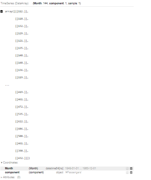
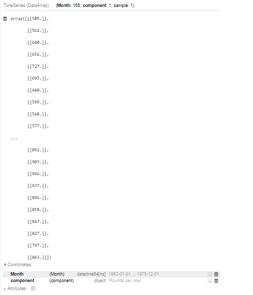
In general, we can load the dataset directly using the load() method, resulting in a mixture of the array and coordinate – Data Array having month datatype as date-time(represents time series).

AirPassengersDataset().load()

MonthlyMilkDataset().load()

Output:

As Dataframe

Alternatively, it can be loaded as a data frame using pd_dataframe().

display("Air Passanger Dataset",AirPassengersDataset().load().pd_dataframe())

display("Monthly Milk Dataset",MonthlyMilkDataset().load().pd_dataframe())

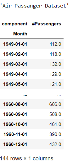
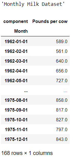
It looks like we have 144 observations for air-passenger and 168 observations for the monthly-milk dataset.

Plotting Datapoints

Dataframe is ok, but It doesn’t reveal much, so we can plot our dataset using matplotlib:

# loading library
import matplotlib.pyplot as plt
%matplotlib inline

# Loading Dataset as Data-Array
air_series = AirPassengersDataset().load() 
milk_series = MonthlyMilkDataset().load()

#plot chart
air_series.plot(label="Number Of Passengers")
milk_series.plot(label="Pounds Of Milk Produced Per Month" )
plt.legend();

In the above code, we just loaded the data and plotted it. Also, we include a label and legend so that it is easy to understand.

The result comes out as a nice looking chart:

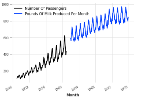
Here x-axis represents the month, and the y-axis – data.

Note you need to downgrade to matplotlib 3.1.3 for code to work in collab.

Data Preprocessing

Carefully observing the above, we can find that the data is not scaled, i.e., it shows variability, so it’s good if we rescale it.

Standard Scaling

Luckily we have Scaler () class for this in the library itself, and we can use it by creating a scaler object and then fitting it to the dataset.

In the above code, we have imported Scaler, created two scaler objects, and performed the scaling.

Now let’s look at the changes to see the difference:

# plottingair_ds.plot(label="Number Of Passengers")
air_series_scaled.plot(label = "Air Passangers Scaled")
milk_series_scaled.plot(label = "Milk In Pounds")
plt.legend();

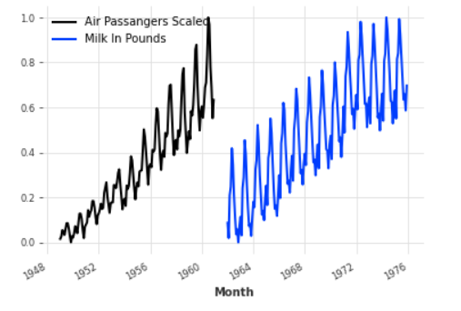
As can be witnessed, our data is scaled and is evident in the plot’s y-axis.

Train Test Split

Now using scaled data, we will split our dataset. For this, we will take the first 36 samples as a training set and remain as a validation set for both datasets.

air_series_train,  air_series_val = air_series_scaled[:-36], air_series_scaled[-36:] 
milk_series_train, milk_series_val = milk_series_scaled[:-36], milk_series_scaled[-36:]

Note this is not a data frame rather a darts time-series object.

For confirming, you can do:

type(air_series_train)

Training the Time Series Model using Darts

Finally, we are in a state to perform the training. DART’s provide many solutions like Arima, Auto-Arima, Varima FFT, Four Theta, Prophet, and a few deep learning models like RNN, Block RNN(Uses LSTM), TCN, NBEATS, Transformer.

Loading the Darts Time Series Model

For our use case, we will go by the N-BEATS model provided as it supports multivariate time series forecasting(data having multiple features), which will allow us to perform all forecasting using a single model. So let’s load it.

# importing model
from darts.models import NBEATSModel
print('model_loaded')

>> model_loaded

NOTE:  you are free to use any model of your liking, but make sure you read the documentation and see each model’s features.

Creating Model Object

Having loaded our model, let’s initiate it.

# creating a model object
model = NBEATSModel(input_chunk_length=24 , output_chunk_length=12, n_epochs = 100 , random_state = 15)

One of the quick things to note here is input, and output chunk length is 24 months and 12 months, respectively. In time series, we usually prefer a window over time instead of using real data. Also, we are doing our training for 100 epochs.

Additional Elaboration

• In the first steps/epoch, we will provide 24 months of data as input data and 12 months as output data.
• In the next step, we will move one step ahead and provide the next 24 months’ data as input and 12 months ‘ output, and so on till all data points of the training set are exhausted.
• Based on this at each step a loss is calculated and the model learns to perform better and better over time.

Fitting Data To Model

Now finally, let’s train our model by fitting our training data. It may take time, so be patient!

# fitting the model
model.fit([air_series_train, milk_series_train], verbose = True)

Verbose = True insures logs.

Prediction and Evaluation of Time Series Model Using Darts

To ensure the model trained is performing well, we can check it MAPE  – Mean Absolute percentage error for the predicted data.

# imports
from darts.metrics import mape

pred_air = model.predict(n = 36, series = air_series_train)
pred_milk = model.predict(n =36, series = milk_series_train)

print("Mape = {:.2f}%".format(mape(air_series_scaled , pred_air)))
print("Mape = {:.2f}%".format(mape(milk_series_scaled , pred_milk)))

Output:

>> Mape = 6.74% 
>> Mape = 16.82%

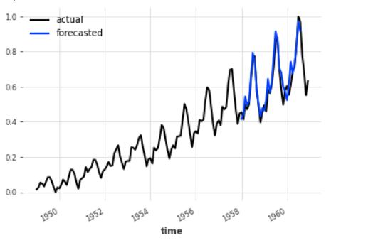
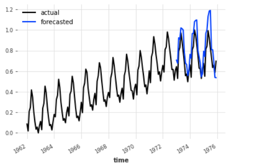
As evident, the errors are quite low, and an interesting pattern emerges that there is somewhat relation between milk produced by cows and the number of air passengers traveling, which is quite interesting. Also, note that we have used a single model to predict both the dataset! (an issue addressed by our boss to fix😁).

Visualization the Time Series using Darts Model Prediction

Finally, let’s look at how our predictions come out on a graph using the same way we checked our dataset but using our scaled dataset for better interpretability.

# plotting results
air_series_scaled .plot(label = "actual")
pred.plot(label = "forecasted") # validation data set
plt.legend()

# plotting results

milk_ds_scaled.plot(label = "actual")

pred.plot(label = "forecasted") # validation data set

plt.legend()

 

The blue line represents the predicted data are very close to actuals(black line). Meaning we have succeeded in our quest and solved the issue addressed in our scenario. Congrats to you!

Conclusion

Some conclusions to derived are:

• Libraries like darts can provide us with a new way to work over time-series, allowing for flexibility and efficiency.

• As evident, we can load, process, and even train multiple datasets using a single library and model.

• With all the charm, one can successfully throne it as a scikit-learn for time series data.

With this, we have come to an end of this miniature article. I hope you have found this interesting and will apply the learned in some of your projects.

See you later.

REFERENCES:

Code Notebook:- Collab

To Connect:-  Linkedin, Twitter, Github, AnalyticsVidhya

All images are by the author.

Purnendu Shukla

24 Oct 2021

Hey All✋,
My name is Purnendu Shukla a.k.a Harsh. I am a passionate individual who likes exploring & learning new technologies, creating real-life projects, and returning to the community as blogs.
My Blogs range from various topics, including Data Science, Machine Learning, Deep Learning, Optimization Problems, Excel and Python Guides, MLOps, Cloud Technologies, Crypto Mining, Quantum Computing.