This article was published as a part of the Data Science Blogathon
What is Model Monitoring and why is it required?
Machine learning creates static models from historical data. But, once deployed in production, ML models become unreliable and obsolete and degrade with time. There might be changes in the data distribution in production, thus causing biased predictions. User behavior itself might have changed compared to the baseline data the model was trained on, or there might be additional factors in real-world interactions which would have impacted the predictions. Data drift is a major reason model accuracy decreases over time.
Thus, monitoring the changes continuously in our model’s behavior is of utmost importance. Flagging such drifts and automating certain jobs for retraining the model with new data or manual intervention of any kind ensures that the model remains relevant in production and gives fair and unbiased predictions over time.
Types of Data Drift
1) Concept Drift
Concept drift means that the statistical properties of the target variable, which the model is trying to predict, change over time. This causes problems because the predictions become less accurate and become unreliable.
Example:
The abrupt changes in consumer behavior brought on by COVID-19 had a major impact on the accuracy of forecasting models that rely on historical data to inform their predictions. This can be treated as an example of concept drift.
One of the main reasons for concept drift to occur is the non-stationarity of data i.e., change in statistical properties of data with time.
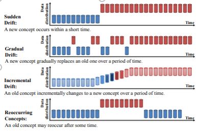
Image source: https://arxiv.org/pdf/2004.05785.pdf
2) Covariate Drift
Covariate shift is the change in the distribution of one or more of the independent variables or input variables of the dataset. This means that even though the relationship between feature and target variable remains unchanged, the distribution of the feature itself has changed. When statistical properties of this input data change, the same model which has been built before will not provide unbiased results. This leads to inaccurate predictions.
Example: Suppose a model is trained with a salary variable that ranges from 200$ to 300$ and is in production. Over time, salary increases and the model encounters real-time data with higher salary figures of 1000$,1200$, and so on. And the model will see an increase in mean and variance, and therefore it leads to a data drift.
Data Drift Detection Framework
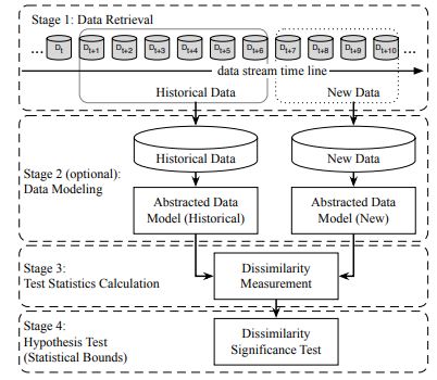
Image source: https://arxiv.org/pdf/2004.05785.pdf
Stage 1 (Data Retrieval) is used to retrieve data from data streams in chunks since a single data point cannot carry enough information to infer the overall distribution.
Stage 2 (Data Modeling) is used to extract the key features, that is, the features of the data that most impact a system if they drift.
Stage 3 (Test Statistics Calculation) is to measure the drift and calculate test statistics for the hypothesis test.
Stage 4 (Hypothesis Test) is used to evaluate the statistical significance of the change observed in Stage 3 or the p-value.
Methods for Detecting Data Drift
All the methods for detecting data drift are lagging indicators of drift. Only after they have processed enough data after any kind of drift that has occurred, that the actual drift is detected.
1) Kolmogorov-Smirnov (K-S) test:
The K-S test is a nonparametric test that compares the cumulative distributions of two data sets, in this case, the training data and the post-training data. The null hypothesis for this test states that the data distributions from both the datasets are same. If the null is rejected then we can conclude that there is adrift in the model.
In our analysis, we have only considered numerical columns for the test.
For generating our final Data Drift analysis, the chi-squared test can be applied for the categorical features to identify data drift.
Python implementation:
df.drop(['RowNumber','CustomerId','Surname'],axis=1,inplace=True)
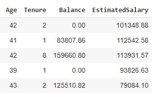
df_numerical=df.iloc[:,[3,4,5,9]]
df_numerical.head()
df_salary_low=df_numerical[df_numerical['EstimatedSalary']<=10000]

#splitting the data to analyze the difference in both the datasets
from scipy import stats

p_value = 0.05

rejected = 0

for col in df_numerical.columns:

    test = stats.ks_2samp(df_salary_low[col], df_salary_high[col])

    if test[1] < p_value:

         rejected += 1

         print("Column rejected", col)

print("We rejected",rejected,"columns in total")

Thus, the K-S test has rejected the Tenure and Estimated Salary columns which means that the statistical properties of these two columns for both the datasets are not identical.
2) Population Stability Index:
It compares the distribution of the target variable in the test dataset to a training data set that was used to develop the model.

Steps for calculation:
1) Divide the expected (test) dataset and the actual (training dataset) into buckets and define the boundary values of the buckets based on the minimum and maximum values of that column in train data.
2) Calculate the % of observations in each bucket for both expected and actual datasets.
3) Calculate the PSI as given in the formula
a) When PSI<=1
This means there is no change or shift in the distributions of both datasets.
b) 0.1< PSI<0.2
This indicates a slight change or shift has occurred.
c) PSI>0.2
This indicates a large shift in the distribution has occurred between both datasets.
def calculate_psi(expected, actual, buckettype='bins', buckets=10, axis=0):
  def psi(expected_array, actual_array, buckets):
        def scale_range (input, min, max):
            input += -(np.min(input))
            input /= np.max(input) / (max - min)
            input += min
            return input
        breakpoints = np.arange(0, buckets + 1) / (buckets) * 100
        breakpoints = scale_range(breakpoints, np.min(expected_array), np.max(expected_array))
        expected_percents = np.histogram(expected_array, breakpoints)[0] / len(expected_array)
        actual_percents = np.histogram(actual_array, breakpoints)[0] / len(actual_array)
        def sub_psi(e_perc, a_perc):
            if a_perc == 0:
                a_perc = 0.0001
            if e_perc == 0:
                e_perc = 0.0001
            value = (e_perc - a_perc) * np.log(e_perc / a_perc)
            return(value)
psi_value = np.sum(sub_psi(expected_percents[i], actual_percents[i])
for i in range(0, len(expected_percents)))
return(psi_value)
  if len(expected.shape) == 1:
      psi_values = np.empty(len(expected.shape))
  else:
      psi_values = np.empty(expected.shape[axis])
  for i in range(0, len(psi_values)):
      psi_values = psi(expected, actual, buckets)
return(psi_values)
## Calculate psi for features
psi_list = []
top_feature_list=df_salary_high.columns
for feature in top_feature_list:
        # Assuming you have a validation and training set
        psi_t = calculate_psi(df_salary_high[feature], df_salary_low[feature])
        psi_list.append(psi_t)
        print('Stability index for column ',feature,'is',psi_t)

3) Model-Based Approach
A Machine Learning-based model approach can also be used to detect data drift between two populations.
We need to label our data which has been used to build the current model in production as 0 and the real-time data gets labeled as 1. We now have to build a model and evaluate the results.
If the model gives high accuracy, it means that it can easily discriminate between the two sets of data. Thus, we could conclude that a covariate shift has occurred and the model will need to be recalibrated. On the other hand, if the model accuracy is around 0.5, it means that it is as good as a random guess. This means that a significant data shift has not occurred and we can continue to use the model.
The disadvantage of this model is that every time new input data is made available, the training and testing process needs to be repeated which can become computationally expensive.
4) Using specialized drift detection techniques such as Adaptive Windowing (ADWIN):
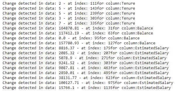
The Adaptive Windowing (ADWIN) algorithm uses a sliding window approach to detect concept drift. Window size is fixed and ADWIN slides the fixed window for detecting any change on the newly arriving data. When two sub-windows show distinct means in the new observations the older sub-window is dropped.
A user-defined threshold is set to trigger a warning that drift is detected. If the absolute difference between the two means derived from two sub-windows exceeds the pre-defined threshold, an alarm is generated. This method is applicable for univariate data.
from skmultiflow.drift_detection import ADWIN
adwin = ADWIN()
for col in df_numerical.columns:
  data_stream=[]
  a = np.array(df_salary_low[col])
  b = np.array(df_salary_high[col])
  data_stream = np.concatenate((a,b))
# Adding stream elements to ADWIN and verifying if drift occurred
  for i in range(len(data_stream)):
    adwin.add_element(data_stream[i])
    if adwin.detected_change():
        print('Change detected in data: ' + str(data_stream[i]) + ' - at index: ' + str(i) +'for column:' + col)
5) Page-Hinkley method:
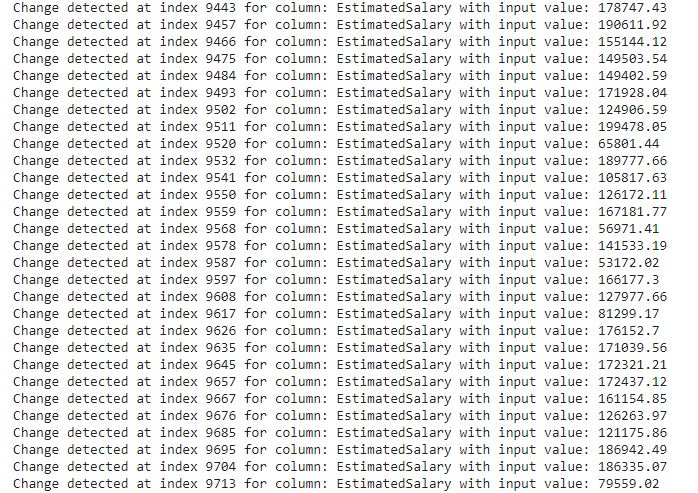
This drift detection method calculates the mean of the observed values and keeps updating the mean as and when new data arrives. A drift is detected if the observed mean at some instant is greater than a threshold value lambda.
min_instances – defaults to 30
The minimum number of instances before detecting change.
delta – defaults to 0.005
The delta factor for the Page Hinkley test.
threshold – defaults to 50
The change detection threshold (lambda).
alpha – defaults to 0.9999
The forgetting factor is used to weigh the observed value and the mean.
from river.drift import PageHinkley
np.random.seed(12345)
ph = PageHinkley(threshold=10,min_instances=10)
# Update drift detector and verify if change is detected
for col in df_numerical.columns:
  data_stream=[]
  a = np.array(df_salary_low[col])
  b = np.array(df_salary_high[col])
  data_stream = np.concatenate((a,b))
  for i, val in enumerate(data_stream):
     in_drift, in_warning = ph.update(val)
     if in_drift:
           print(f"Change detected at index {i} for column: {col} with input value: {val}")
Handling data drift in production
In production, there are multiple ways to respond to data drift.
Some of the methods which are generally followed in the industry are:
1) Blindly update model:
This is a naïve approach. There is no proactive drift detection. Models are periodically retrained and updated with recent data. Without drift detection in place, it is difficult to estimate the time interval for re-training and model re-deployment.
2) Training with weighted data:
When a new model is trained instead of discarding old training data, use weight inversely proportional to the age of data.
3) Incremental learning:
As new data arrives, the models are continuously retrained and updated. As a result, the model is always adapting to the changes in the data distribution. This approach will work with machine learning models which allow incremental learning one instance of data at a time.
Conclusion
There are various ways to detect and handle drift. Custom alerts and thresholds can be also set up by the user to trigger alerts for drift. In Cloud platforms e.g in Azure Machine Learning, you can use dataset monitors to detect and alert for data drift.
Thus, Model Monitoring and Drift Detection is an important part of the ML Model Lifecycle which needs to be optimized for successful and efficient deployments of models into production. Identifying any kind of drifts in the data in real-time and a proper strategy to handle such drifts is very crucial for our models to give better results with time.


