The Complete Guide to Checking Account Churn Prediction in BFSI Domain

This article was published as a part of the Data Science Blogathon.

Table of Contents

1. What is a Checking Account & Its importance to Financial Institutions?
2. Data Requirements for building Churn Prediction model
3. Defining what Churn means to a FI
4. Defining Static Pool and Time frame for Independent & dependent (Target) Variable
5. Generating Independent variables & Dependent Variable
6. Applying Exclusions & Segmented model
7. Model Building & Validation
8. Model Evaluation
9. Segmentation Strategy and Model Application
10. End Notes

What is a Checking Account & Its importance to Financial Institutions?

A checking account is a bank account where customers deposit money which can be utilized for writing checks, wire transfers, make payments with Debit Cards, and receive salaries via direct deposits by the employers. It offers a low interest on the deposited amount but the ones with a higher deposit maintenance balance have a higher rate of interest.

Fees are also charged on these accounts if the balance falls below the stipulated balance amount which brings some income to the Financial Institutions (FIs). More than the fee income, FIs care about having an active relationship in Checking product.

Customers initiate their relationship with Financial Institutions (FIs) like large banks, credit unions by opening their Checking Account as their first banking product. The financial institutions can then strengthen their relationship by cross-selling other banking products like Credit Card, Personal Loan, Mortgage, Certificate of Deposits, IRA, etc. Therefore, the FIs need to engage these customers, and proactively retain them. One strategy that is commonly followed by FIs is to predict in advance the customers likely to churn in the coming months.

This article will talk about what factors should be taken into account while building a Churn prediction model, understand how to build the dataset and the model, evaluate the performance of the model, and how can FIs build some effective tactics with the output of the model using Segmentation

Data Requirements

Broadly, the following data can be utilized for preparing the analytical dataset for the model:

1. Customer Demographics– Customer related details like Age, Months on book, city, Gender, Profession, Income
2. Customer Product Relationships– Information regarding other products held by the customer like Personal Loans, Credit Cards, Mortgage, etc. It includes no. of products, balances, product sub-types, etc.
3. Product Transactions– data related to transactions in different products including deposits, withdrawals, transaction value, debit & credit, ATM, Debit Card, Online Banking Transactions, etc.
4. Customer Interactions– data related to the interaction of customers with the bank through different channels like Call Centre, Email, Direct Mail
5. Bureau data-Bureau data provides attributes of how customers deal with other FIs. Data such as FICO score, number of revolving products(Credit Card, HELOC) held, delinquency status, payments made come under this category
6. Digital Tracking data– With digital in focus these days, FIs have started tracking customer interactions on their website, blogs, and mobile app. Data points such as Page Visits, Clicks on CTA buttons, Clickstreams can be used in this context

Once all the above-mentioned data is available, consolidate it into master data at the customer level with granularity at the monthly or weekly level. The consolidated master data may look as follows (Fig 1.1).

Once the master data is prepared, we can move ahead with the time frame selection for model building and model validation. We would need data of at least 24 months to build and validate our model. Suppose we have the data available from Jan’ 2015 through Jun’2020. We can use the period from Jun’ 2018 to Dec’ 2019 for model building and the period from Jan’20 to June’20 for model Validation. It is generally a good practice to validate the model on the latest pool of available data.

Once we have the required data for the selected time frame, we start building our independent variables and the dependent variable.

Definition of what Churn means to a FI

To build our dependent variable, we need to define what churn means for a checking account customer. The definition can vary from customers who have been inactive in the checking account for the last 12 months to customers who have closed their checking accounts. The definition should be consistent with the business/client’s requirements. In our case, we can define churn customers as those who closed their checking accounts.

Let us understand how to create our independent and dependent variables.

Defining Static Pool and Time frame for Independent & dependent (Target) Variable

The static pool is the month of the year which is used as a reference point to define our Observation and Performance Window. An example of a static pool in our case will be the set of all customers holding a Checking account as of a particular month (201712).

We define two windows here: The observation window and the Performance window. The window during which we create our independent variables is known as the Observation window whereas the time duration where we create our target variable is called as Performance window.

It is to be noted that the performance window is ahead of the static pool month and the observation window is at the back of the static pool month. Look at Fig. 1.2, we had 2 customers A and B both of them holding a checking account as of 201712. However, customer A has attrited after 6 months during the performance window whereas customer B is still with the FI.

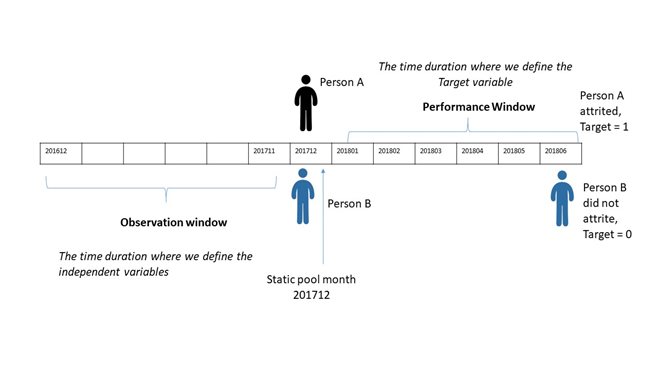
Fig 1.2 Defining Observation and Performance Windows

It is important to note that the length of observation and performance windows depends on many factors some of which are mentioned below:

1. Availability of data: If the data is available for a smaller period, we can reduce the length of both the windows. However, it is always desirable to build a model on a large sample of data
2. The event rate during the performance window: Event rate is defined as the number of customers attrited divided by the total number of checking customers in the static pool. Less number of customers would attrite in 1 month as compared to 6 months. To build a good model, a higher event rate is desirable
3. Seasonality in the data: Certain months of the year would have higher attrition as compared to other months. We would want to cover the period with seasonal variations
4. Reactiveness in dealing with Customers likely to churn: FIs may want to curb the customer churn proactively. In such cases, the Performance Window should be chosen small to predict the attrition early

Sometimes, it makes more sense to include multiple static pools while building model data. This is preferred when different static pools have different event rates in the performance window. It will allow the model to capture the variability in event rates across different months of the year.

Suppose we decide to keep the length of the observation window as 12 months and for the performance window as 6 months, we can then select our static pools by analyzing the 6-month rolling attrition rate as given in Fig 1.3. It has a 6-month forward attrition rate for each of the months from the Year 2015 through 2020.  We can select our static pools as months having the lowest and highest 6-month attrition rate in the first two and the last two quarters of the year 2019. Based on the table, we can decide to choose year month 201912, 201907, 201905, and 201903 as our static pools.

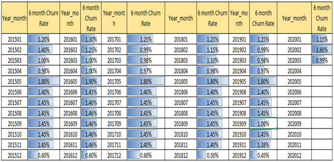
Fig 1.3 6-Month Rolling Attrition

Once we decide on the appropriate static pools, we start the data preparation by creating the independent and dependent variables for each of the static pools. Once we have all the data, we append all the static pool to get our final model building data.

Let us consider one static pool 201912 and see what variables we can make.

Generating Independent variables & Dependent Variable

Broad categories of Independent variables can include Demographics, Product information, Transaction in products, Interactions & Bureau variables. To give an idea of the type of variables that we can create, refer to the table in Fig 1.4

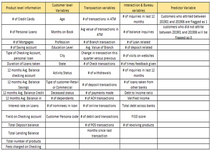
Fig. 1.4 Independent & Dependent Variables

Applying Exclusions & Segmented model

Once our analytical dataset is ready to build the model, certain exclusions can be applied to remove the customers which FIs do not want to target. For example, Excluding customers who are new to the bank can be excluded because they would not have the data for the past 12 months. Other exclusions may include student accounts, business accounts, etc.

Sometimes instead of excluding the new customers, FIs may decide to create a separate model for those customers. This is called a Segmented model approach where segments of the population having different characteristics are targeted with different models. An example of a segmented approach could be creating segments based on FICO Score. Customers with lower FICO scores have a different profile as compared to the customers with a higher FICO score.

 Model Building & Validation

The Dependent variable in our case is a binary categorical variable having values as 0 and 1. We can think of applying a binary classification Machine Learning technique like Logistic Regression to build the model. You can read about the implementation of Logistic Regression here.

Before building the model, divide the data into two parts: Build and Validation sample. Typically we divide the data in a ratio of 75: 25. We use 75% of the data for building the model and 25% of the data is used for Validation. The validation done at this stage is also called In-time Validation since the data belongs to our chosen static pools. When we validate the model on a different static pool, we call it is Out of time (OOT) validation. OOT Validation should be done on the latest available data and the model should perform consistently on the evaluation metrics on OOT as well.

Sometimes we also try to validate the model on static pools belong to a long history or periods having abnormal event rates (Black Swan events like Corona, Recession of 2007). This process is known as backtesting of models which is generally done for models in the Risk space.

While dividing the dataset we need to ensure that both the build and validation sample have the same event rate. Stratified Sampling is used to ensure an equal event rate between the build and validation sample.

When the event rate is small in our build sample, we can use techniques like SMOTE or TomekLinks, class_weight/scale_pos_weight hyperparameters to increase the event rate. You can read more about these techniques here.

Some of the levers that affect Checking account attrition include:

1. Average Checking Balance of last 3 months ( higher balance leads to lower attrition)
2. Total number of transactions ( ATM/Check/POS transactions) done in the last 6 months (higher the total transactions, lower the chances of attrition)
3. The total amount of fees charged in the last 3 months ( higher the fees charged, higher the chances of attrition)
4. Total number of Enrolments in digital services ( higher the enrolment, the lower chances of attrition)
5. Type of Checking account ( Premium checking customers have low chances of attrition)
6. Presence of Mortgage Product ( The presence of Mortgage with the customers leads to low attrition in Checking)

Model Evaluation

We can evaluate our model performance using multiple metrics like Kolmogorov-Smirnov statistic (KS), Lift to check how well the model performs as compared to a Random selection. The evaluation metrics should remain consistent on both the build and validation samples.

The output of Logistic Regression is a probability value between 0 and 1 which tells us the chances of a customer attriting in the next 6 months. We create deciles based on the probability value and count the number of events and non-events in each decile. Based on that, we generate the following tables for both the build and test samples in Fig 1.5 and Fig 1.6 respectively.

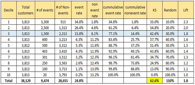
Fig 1.5 Evaluating model on Build Sample

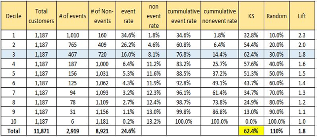
Fig 1.6 Evaluating model on Validation Sample

From the above figures, we can see that the top 3 deciles cover approximately 77% of the customers which have higher chances of attrition in the next 6 months. FI’s can simply target these customers instead of focussing on all the customers. This will also reduce the cost of targeting for the banks.

We can see that model performs consistently well on the validation sample as well. It has approximately the same value for KS and Lifts across all the deciles for both the build and validation samples. The value of KS statistic (maximum across all deciles) lies within the top 3 deciles for both the samples.

To compare the model performance with the random selection, we look at the Lift and the Cumulative accuracy profile is given in Fig 1.7. The model built shows a significant lift (Blue Line) over the random selection line (Orange Line).

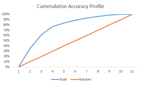
Fig. 1.7 Cumulative Accuracy Profile

You can read more about KS, Lift, and Cumulative Accuracy Profile here.

Segmentation Strategy and Model Application

Once the model is built we calculate the probability of attrition for the current pool of customers holding a checking account. We can then perform Segmentation on customers based on dimensions like Product holding, total profits earned in the last 12 months, and the probability of attrition. It is important to understand the profiles of each segment to create actionable tactics that can prove fruitful in reducing Checking account attrition. Fig 1.8 gives a simple segmentation strategy that FIs can follow.

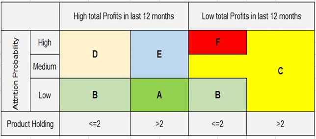
Fig 1.8 Simple Segmentation

Some of the actions that FIs can take for each of the segments are-

Segment A: This segment is the most loyal to the Financial Institution. FIs should make efforts to keep these customers happy. They can be assigned Senior Relationship Managers to handle their queries.

Segment B: This segment should be educated about different product and service offerings by the FIs. Efforts should be made to enroll these customers in digital services. Up-sell different products to these customers. Consider upgrading their Checking accounts, Credit Cards.

Segment C: This segment should be given a significant amount of efforts to increase their share of wallet. Offer Product bundling schemes to increase their balances drive higher usage of credit/debit cards. Triggers should be created for these customers to cross-sell products and enrolment in digital services when a certain action is observed for these customers

Segment D: The segment has low product holding but FI is still earning a good amount of money from this segment. This could be due to the higher amount of fees charged on the Checking account, loan service fees. Efforts should be made to refund fees if the fee is the main concern for leaving the FI. Automated triggers should be sent to these customers when their balance drops below a certain threshold which avoids balance maintenance fees on accounts

Segment E: This segment gives higher profits to the bank and at the same time their product holding is good but still wants to attrite. The reason could be that their queries are not handled on a timely basis or they want better customer service. Assign Junior Relationship Managers to manage them

Segment F: This segment should be given the least attention as they perform the worst on all the parameters. FIs can send reminders of account closure due to inactivity

The last step involves operationalizing the model in an automated environment which would give the list of customers highly likely to attrite every month and following the tactics as defined for each segment

End Notes

In a highly competitive & changing macroeconomic environment where it is difficult to lure customers with better interest rates, the FIs must direct their efforts towards retaining the existing customers and provide good quality service to them.

Needless to say, the FIs should not rely solely on predictive models in their efforts to retain customers. Training employees on how to effectively communicate with customers about products and services and handling customers keeping their needs in mind would help form a lasting relationship with them.

Thanks for reading the article and happy learning? Do let us know your thoughts about this guide in the comments section below.

Himanshu Koli

14 Dec 2020