This article was published as a part of the Data Science Blogathon
Introduction
Identifiability is a very important property of statistical parameters. To understand identifiability, it’s important to revise the basics of statistical modeling.
Statistical modeling is the process of using observable data to capture the truth or the reality. Of course, it’s not possible to capture the entire truth. So, the goal of statistical modeling is to understand as much reality as possible.
There are three fundamental aspects of statistical modeling- estimation, confidence intervals, and hypothesis testing.
Estimation is the process of finding the value of the parameters that characterize the distribution of a random variable. For example, we can say that the estimated effectiveness of a drug is 75%.
Confidence intervals
are used to produce an error bar around the estimated value. For example, we can say that we are 95% confident that the effectiveness of the drug lies between 68% and 81%.
And finally, hypothesis testing– the basis of data-driven scientific inquiry- is used to find a yes/no answer with respect to the underlying distribution. For example, we can say that the null hypothesis that the drug has no effect has been rejected with 99% confidence.
A statistical model for a random experiment is the pair:

Where,
E refers to the measurable sample space of the experiment.
ℙθ refers to the family of probability measures on E i.e., the probability distribution of the random variable assigned to the experiment.
θ refers to the set of unknown parameters that characterize the distribution P.
Θ refers to the parameter space i.e., the set of all possible values that can be assigned to a parameter.
As an example, consider the experiment of the tossing of a biased coin. Let X be a random variable that takes the value 1 in the case of head and 0 in the case of tails. The sample space of the experiment has only 2 possible outcomes: 0 & 1. So, E = {0, 1}.
Clearly, X has a Bernoulli distribution. So ℙ θ = Ber(p), where p is the parameter θ that shows the probability of getting a head. If the coin was unbiased, p would be 0.5. But, for a biased coin, p can take any value in the [0, 1] interval. This is the parameter space of the event. Thus, our statistical model can be represented as:

Most of the statistical modeling that happens around us assume two things:
1) The model is well specified:
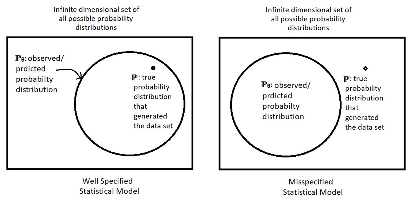
This means that there exist θ such that ℙ θ = ℙ. In other words, there is a particular value/vector in the parameter space which, when plugged into the observed distribution of the random variable (representing a statistical experiment) gives the true distribution of the random variable. The following figure illustrates the concept of specified statistical models:
2) Identifiability of parameters:
This is the concept that we’ll try to explore in this article. Before understanding identifiability, it’s imperative to revise the concept of injectivity because these two ideas (identifiability & injectivity) are very similar.
Injectivity of Functions
Mathematically, an injective function is defined as follows:

In other words, an injective function cannot give the same output for two different inputs. Same outputs can be obtained only by using the same inputs. If we get the same output for two different inputs, then the function is not injective. Let us see a few examples:
1) Is the function f(x) = x2 injective for –∞ < x < ∞?
No. Notice that both -2 & +2 give the same output 4. Hence, it’s not injective.
2) Is the function f(x) = sin(x) injective for 0 ≤ x ≤ π?
No. Notice that both π/6 & 5π/6 give the same output 1/2. Hence, it’s not injective.
3) Is the function f(x) = x2 injective for 0 < x < ∞?
Yes. For every output, we have a unique input. No two inputs give the same output. It can be shown as follows:

As
we don’t have any negative numbers in our domain,

Hence, it’s an injective function.
4) Is the function f(x) = sin(x) injective for 0 ≤ x ≤ π/2?
Yes. For every output, we have a unique input. No two inputs give the same output. It can be shown as follows:

Hence, it’s an injective function.
Now that we have revised the concept of injectivity, we can proceed to understand the idea of the identifiability of statistical parameters.
Identifiability
Identifiability, in simple words, means that different values of a parameter (from the parameter space Θ) must produce different probability distributions. Mathematically, a parameter θ is said to be identifiable if and only if the map,

is injective. That is, for two different values of a parameter (θ & θ’), there must exist two different distributions (ℙ θ & ℙ θ’). That is,

Equivalently (by contraposition),

A non-identifiable parameter on the other hand is one that gives the same distribution for different values that it takes from the parameter space. That is,

Why is the idea of identifiability so relevant?
The identifiability of a parameter allows us to obtain precise estimates for the value of that parameter. In the absence of identifiability, even with an infinite number of observations, we won’t be able to estimate the true value of the parameter θ.
Examples
Example 1
We’ll again take the example of the coin toss. As discussed earlier, the statistical model for the experiment can be represented as follows:

We’ll now check if the parameter ‘p’ of the above model is identifiable or not. To do so, we’ll use the method of contradiction. We’ll first assume that for two different parameters p and p’, we have the same distribution ℙp = ℙp’. The distributions can be shown as:

Now, by assumption:

Thus the parameters p and p’ are equal, which contradicts our assumption that they are different. Consequently,

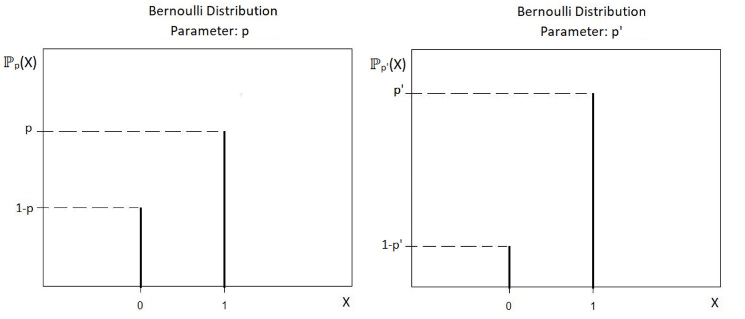
This proves that the parameter p of the given statistical model is identifiable. The variation of ℙp with the value of p has been shown below:
Example 2
We’ll take another example of an identifiable parameter. Consider a random variable X having a normal distribution with mean µ and variance σ2. The sample space of the statistical model will be the entire set of real numbers (–∞, ∞). The statistical model for the example is shown as:

For this model, we’ll prove that the parameters µ and σ are identifiable. Just as before, assume that for two different parameter sets (µ, σ) and (µ’, σ’), we have the same distribution ℙ(µ, σ) = ℙ(µ’, σ’). The distributions can be shown as:

Now, by assumption:
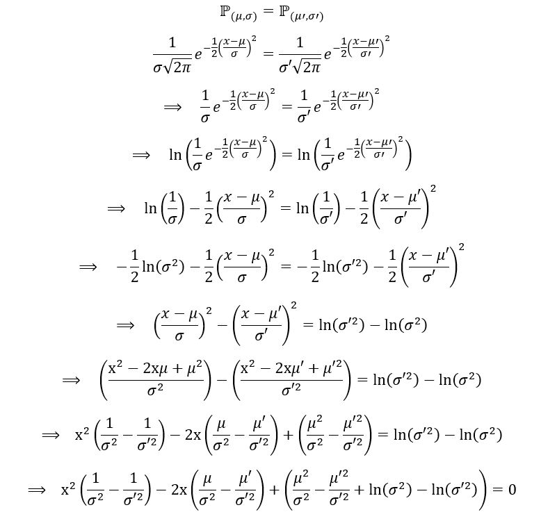
For the above expression to equal zero, it’s important that the coefficient of x and x2 are both zero. Thus,
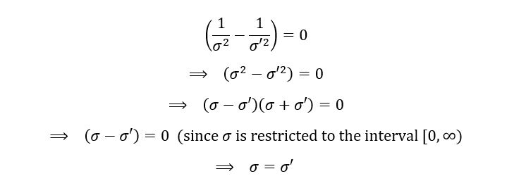
Also,

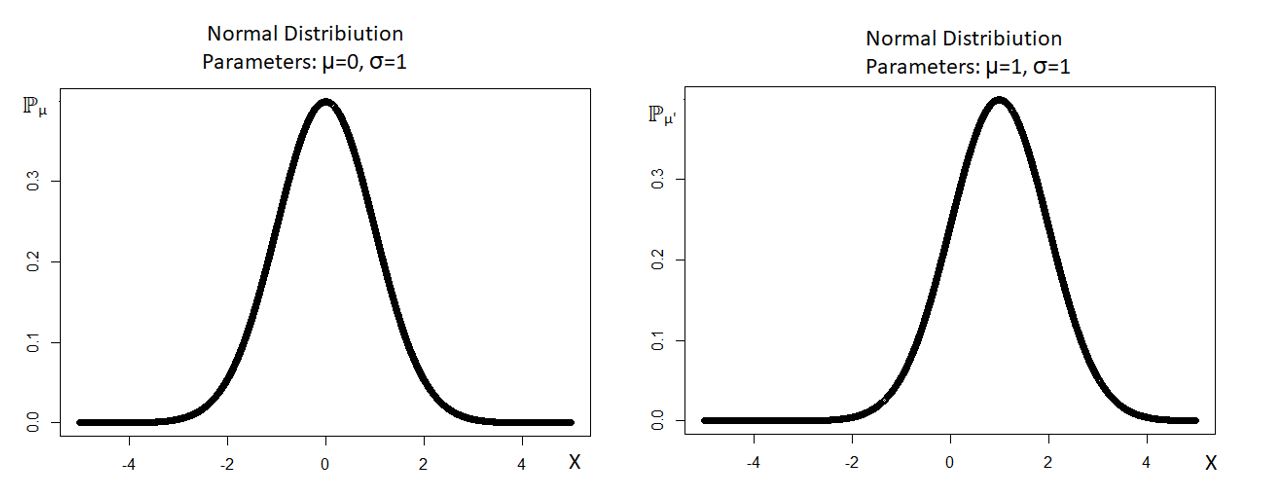
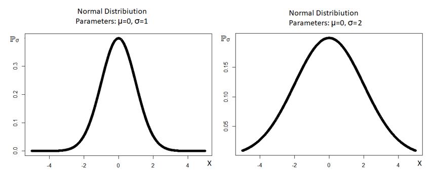
This proves that the parameters µ and σ of the given statistical model are identifiable. The variation of ℙµ with the value of µ has been shown below:
The variation of ℙσ with the value of σ has been shown below:
Example 3
In this final example, we’ll try to understand non-identifiable parameters. We’ll again use a random variable X, which has a Bernoulli distribution. However, we’ll define X in a different way. Let X be defined by the indicator function as follows:

Let p be the parameter of the distribution of X (ℙp). Since X has a Bernoulli distribution, its probability mass function is shown as:

Here, parameter p shows the probability that Yi (having a normal distribution with mean µ and variance σ2) is non-negative. That is,

We follow the process of standardization to obtain Z (the standard normal distribution, having mean 0 and variance 1) as follows:
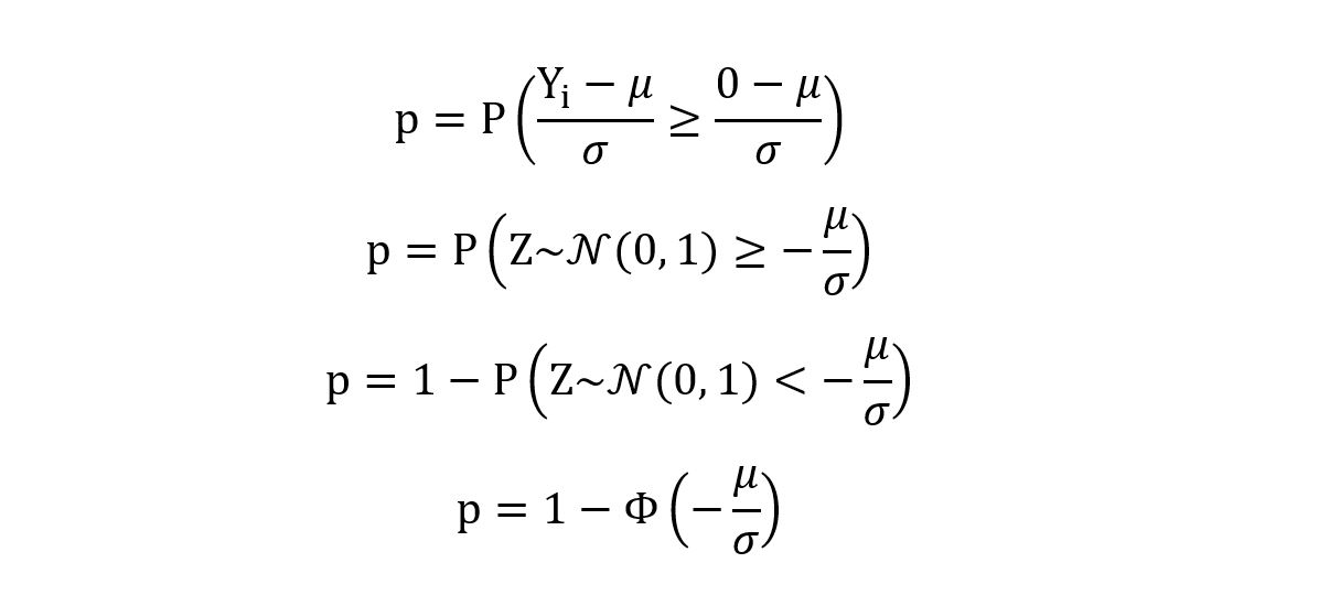
Here, Φ is the cumulative distribution function (CDF) of the standard normal distribution. It can be inferred that the value of the parameter p depends only upon the value of the parameter θ = µ/σ. For this distribution, the parameter set (µ, σ) is non-identifiable. To elucidate this, we’ll take 2 different values for (µ, σ) and show that the distribution of Xi remains the same for both of those values:
First, let the value of (µ, σ) = (1, 2). Thus, the value of p is calculated as:

Next, let the value of (µ, σ) = (2, 4). Thus, the value of p is calculated as:

Hence the value of p remains the same even if the set (µ, σ) takes different values (as long as they are proportional). Consequently, the distribution of Xi remains the same. This shows that the set (µ, σ) is a non-identifiable parameter for the distribution. It’s important to note that while (µ, σ) is non-identifiable, the parameter θ = µ/σ is identifiable for the given distribution (because as µ/σ changes, the value of p changes, which changes the shape of the distribution as p is identifiable).
Conclusion
We started by understanding the formulation of statistical models and the inherent assumptions constituting them. The idea of identifiability was thoroughly discussed in this article using mathematics, theory, and examples.
In case you have any doubts or suggestions, do reply in the comment box. Please feel free to contact me via mail.
If you liked my article and want to read more of them, visit this link.
About the Author

The media shown in this article on K-Means Clustering Algorithm are not owned by Analytics Vidhya and is used at the Author’s discretion.


