Introduction
It’s a well-known fact that we spend too much time on data preparation and not as much time as we want on building cool machine learning models. In fact, a Harvard Business Review publication confirmed what we always knew: analytics teams spend 80% of their time preparing data. And they are typically slowed down by clunky data preparation tools coupled with a scarcity of data science experts.
But not for much longer, folks! RapidMiner recently released a really nice functionality for data preparation, RapidMiner Turbo Prep. You will soon know why we picked this name 🙂, but the basic idea is that Turbo Prep provides a new data preparation experience that is fast and fun to use with a drag and drop interface.
Let’s walk through some of the possibilities of this feature, as well as demonstrate how it integrates with RapidMiner Auto Model, our automated machine learning product. These two features truly make data prep and machine learning fast, fun, and simple. If you would like to follow along, make sure you have RapidMiner Studio 9.0 downloaded. All free users have access to Auto Model and Turbo Prep for 30 days.
Table of Contents
- Loading and Inspecting the Data
- Transforming Data
- Viewing the Process
- Predicting Delays using Automated Machine Learning
- Data Preparation and Machine Learning Simplified
Loading and Inspecting the Data
First, we’re going to start by loading some data. Data can be added from all repository-based sources or be imported from your local machine.
RapidMiner Turbo Prep start screen
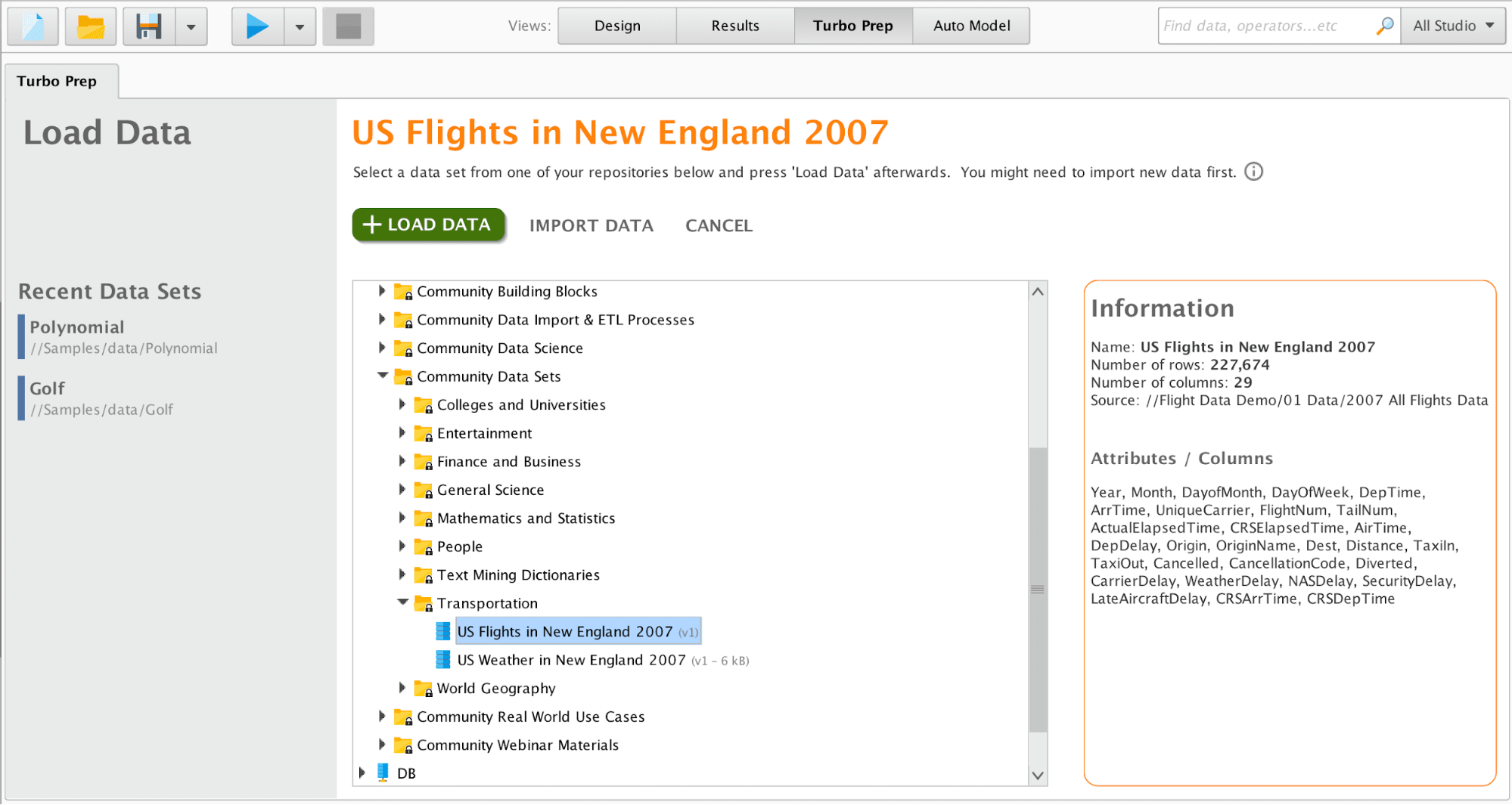
In this example, we’re using a dataset of all the domestic flights leaving from New England in 2007, roughly 230,000 rows. You can find this dataset inside Studio’s pre-installed repository. Click ‘Load Data’ / ‘Community Samples’ / ‘Community Data Sets’ / ‘Transportation’.
Loading sample data sets
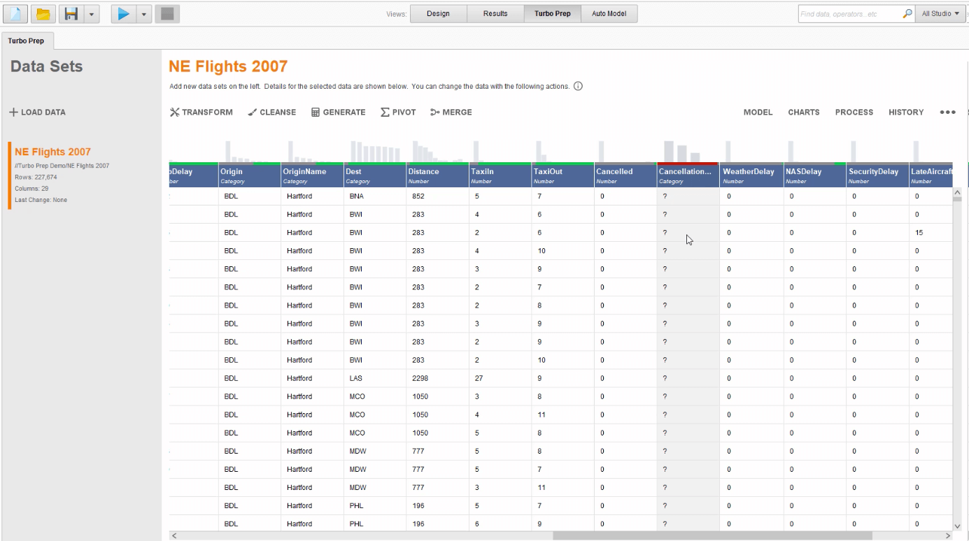
Once you load the data it can be seen immediately in a data-centric view, along with some data quality indicators. At the top of the columns, the distributions and quality measurements of the data are displayed. These indicate whether the columns will be helpful for machine learning and modeling. Say, for example, the majority of the data in a column is missing, this could confuse a machine learning model, so it is often better to remove it all together. If the column acts as an ID, that means practically all of the values only occur once in the data set, so this not useful for identifying patterns, and also should be removed.
Data centric view of RapidMiner Turbo Prep
Transforming Data
Pivot Tables
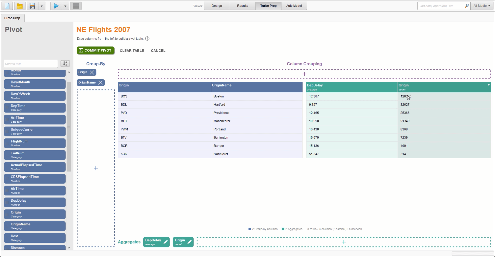
As a first step, in order to look at the data in aggregate, we are going to create a pivot table. To generate this pivot table, first, we will look at the airport codes, indicated by ‘Origin’, with the airport name ‘OriginName’, and calculate the average delay at these locations. We can see the result immediately by dragging ‘DepDelay’ into the ‘Aggregates’ area, which calculates the average. In this case, the biggest delays are happening at the Nantucket airport, which is a very small airport; there is a high average delay of more than 51 minutes. In order to take the number of flights into account, we will also add in ‘Origin count’ and sort to show the largest airport by flight. In this case, Boston Logan Airport is the largest with almost 130,000 flights.
Pivot table in RapidMiner Turbo Prep
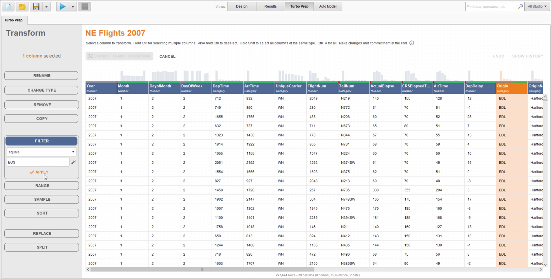
This pivot table helped us quickly determine that we should focus on Boston Logan, so we will exit out of this view and go back to the original data we started with. Now, to only show ‘BOS’ flight data: select the ‘Origin’ column, right click, and select ‘Transformations’, then ‘Filter’. Immediately, there will be a preview of the data, so you know whether the results are correct. All the statistics and quality measurements are updated as well.
Applying a filter
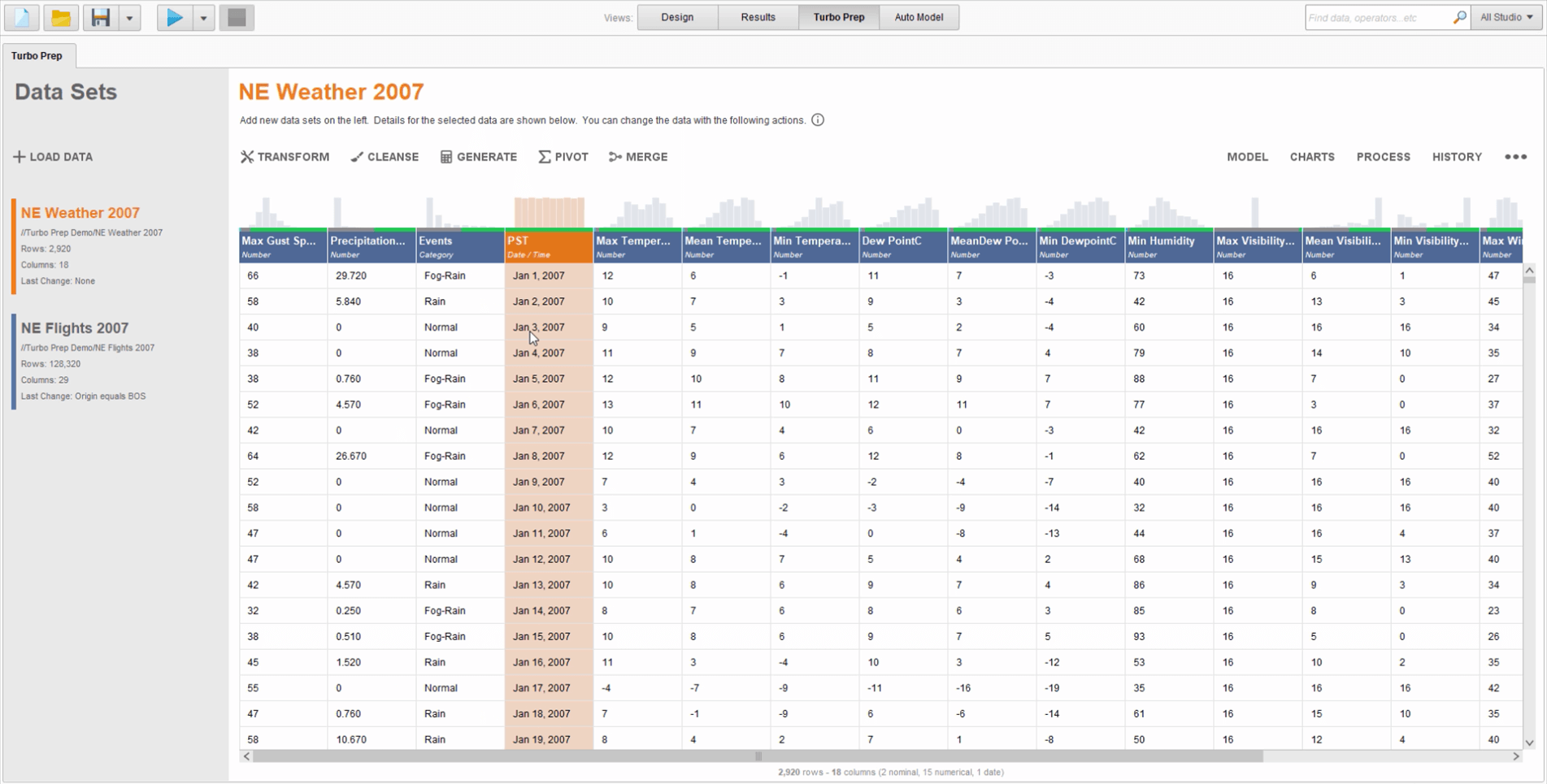
Next, we’re going to bring in some additional data about the weather in New England for the same year. This data set can be found in the same ‘Transportation’ folder as the flight data. We know from personal experience, that weather can create delays, so we want to add this data in to see if the model picks up on it. In a longer scenario, we might take a look at the flight data alone at first and discover that the model is 60% accurate. Then add in the weather information and see how the accuracy of the model improves. But for this demonstration, we will go straight to adding in the weather. In this data, there is a single ‘Date’ column but in our flight data there were two columns, one for the day and one for the month, so we’ll need to transform the weather data to match.
Single ‘Date’ Column in weather data
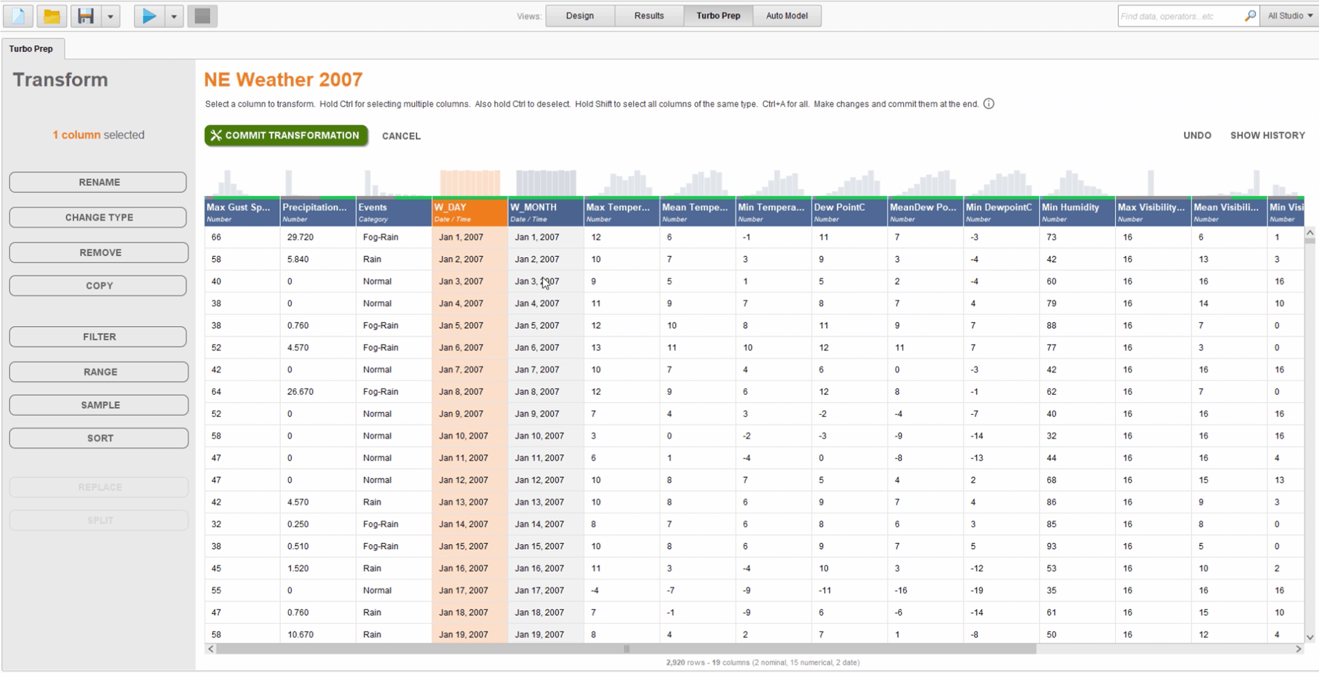
Start the transformation by copying the ‘Date’ column so there are two duplicate columns next to each other. Then rename the columns to ‘W_Day’ and ‘W_Month’ for consistency.
Copied and renamed ‘Date’ columns in weather data
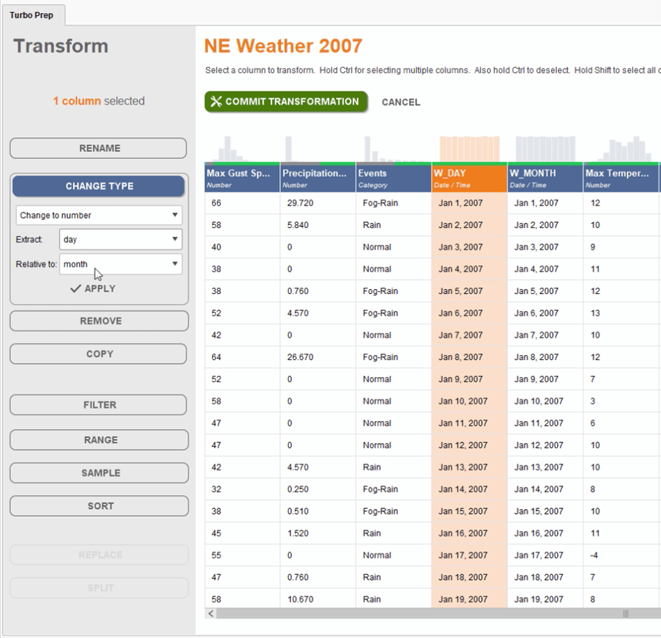
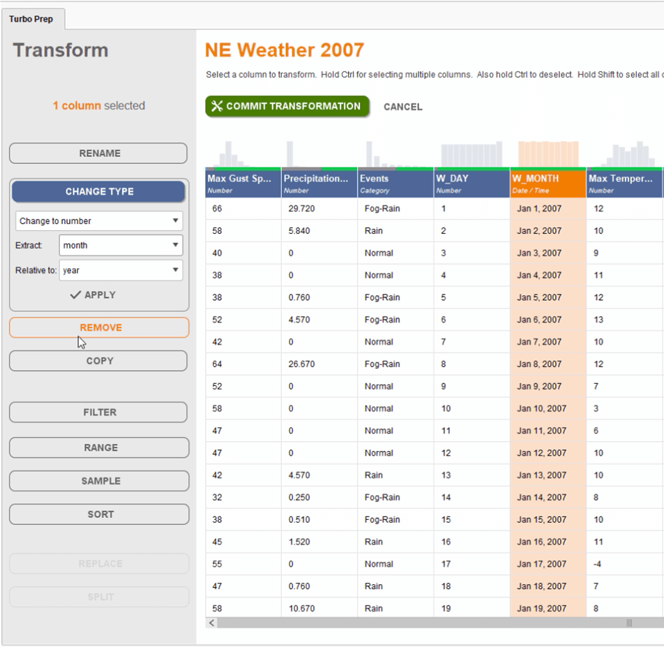
Then we need to split the data from these columns. To do so, click on the ‘W_Day’ column and select ‘Change Type’ which will display ‘Change to number’ with the option to ‘Extract’. In this case we need to extract the day relative to the month and click ‘Apply’. In the case of the ‘W_Month’ column, we need to follow the same steps, except we need to extract the month relative to the year and click ‘Apply’. Once the results look good, we commit the transformation.
Extracting the day from the month
Extracting the month from the year
Merging data
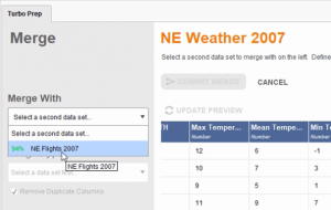
Now, we need to merge the two data sets together. Turbo Prep uses smart algorithms to intelligently identify data matches. Two data sets are a good match if they have two columns that match with each other. And two columns match well with each other if they contain similar values. In this example, we see a pretty high match of 94%.
% match of the two data sets
Joins
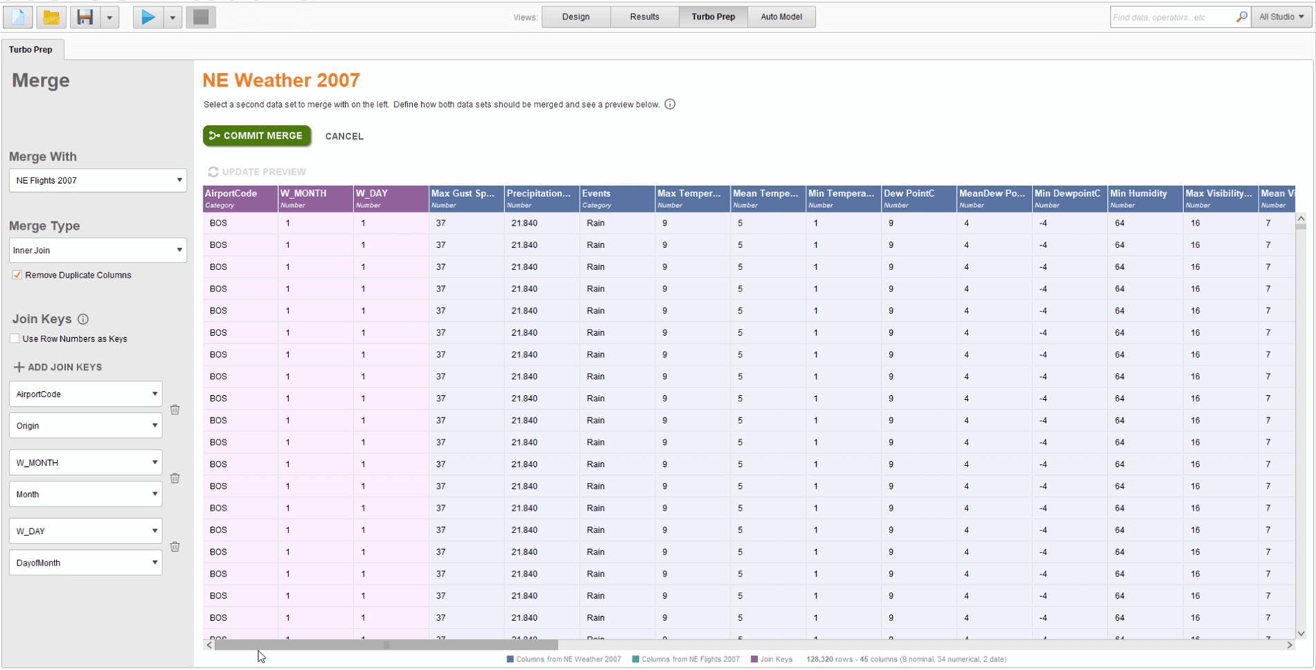
Now if we would like to join on the airport code, we select merge type ‘Inner Join’ and ‘AirportCode’ from the dropdown, and it ranks the best matching columns. The best match is the ‘Origin’ code column in the other data set, which is a good sign. Next, we pick the month and the month pops up to the top showing it’s the best match. Last, we select day and ‘DayofMonth’, which is at the top of the list as the best match. This is helpful to make sure that the joins and merges deliver the correct results. Clicking ‘Update preview’ will show us the three joined keys in purple, all of the weather information in blue, and all of the original flight information for Boston Logan in green.
Merged data view
Generating columns
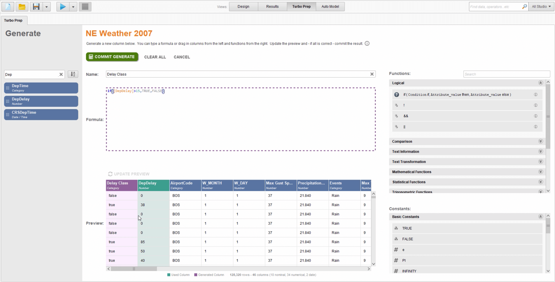
Next, we will generate a new column based on existing information in our data sets. The data in the ‘DepDelay’ column indicates the number of minutes the flight was delayed. If a flight is a minute late, we would not (for this purpose) actually consider that to be delayed so this column, as is, isn’t all that important to us. What we want to do is use this column to define what a delay is. For this example, we will consider any flights more than 15 minutes late as a delay. To generate this new column, we will click ‘Generate’ and will start by creating a new column called ‘Delay Class’. Next, we can either drag in or type out, the formula of ‘if()’. The drag in, or type out ‘DepDelay’ where a delay greater than fifteen minutes is true, and the rest is false. Ultimately, the formula will read, ‘if([DepDelay]>15,TRUE,FALSE)’. Then, we want to update the preview to see the amount of false versus true. In our case, the formula seems to work, so we commit the Generate and the new column is added.
Generating a ‘Delay Class’ column
Cleansing data
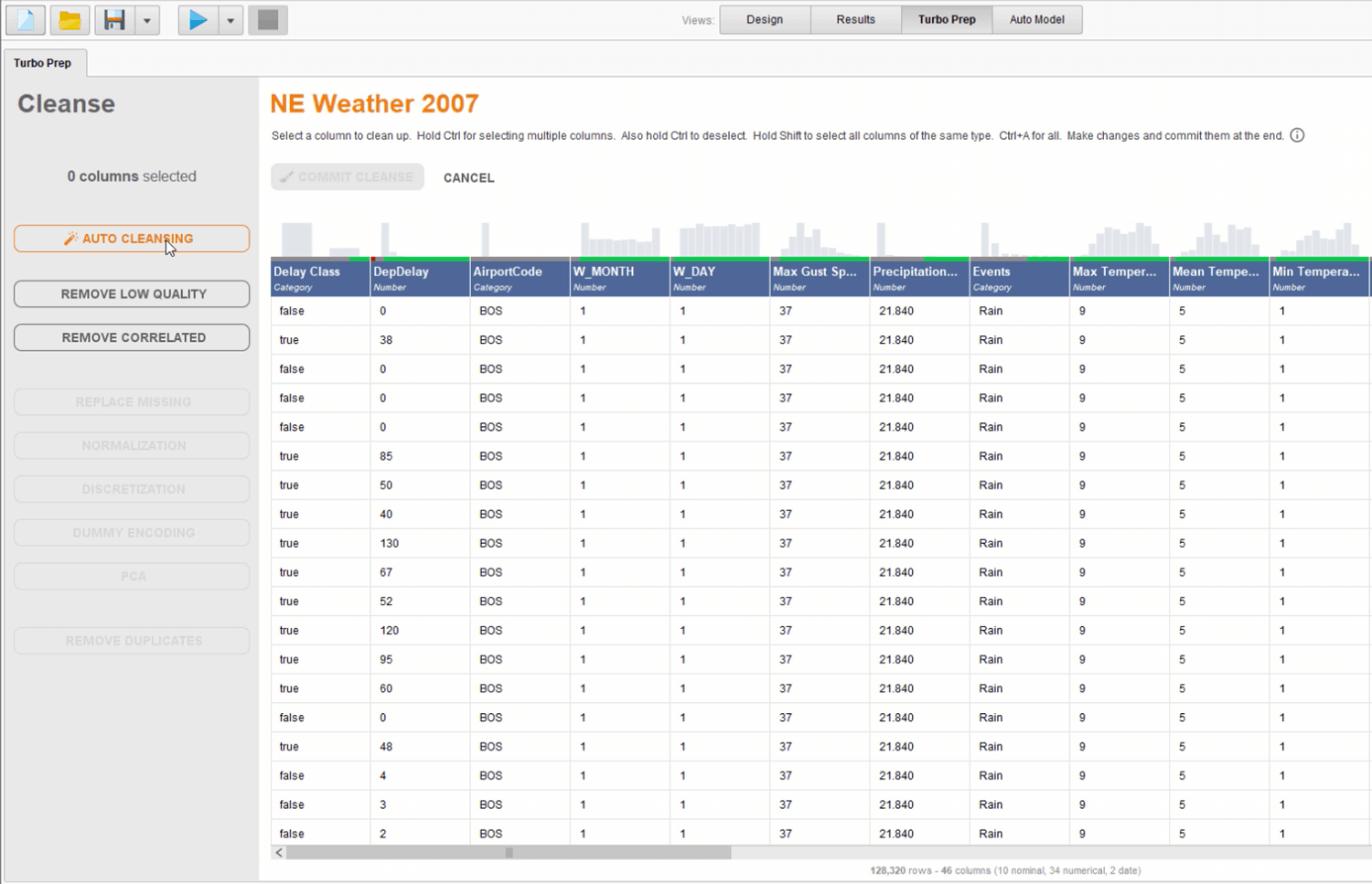
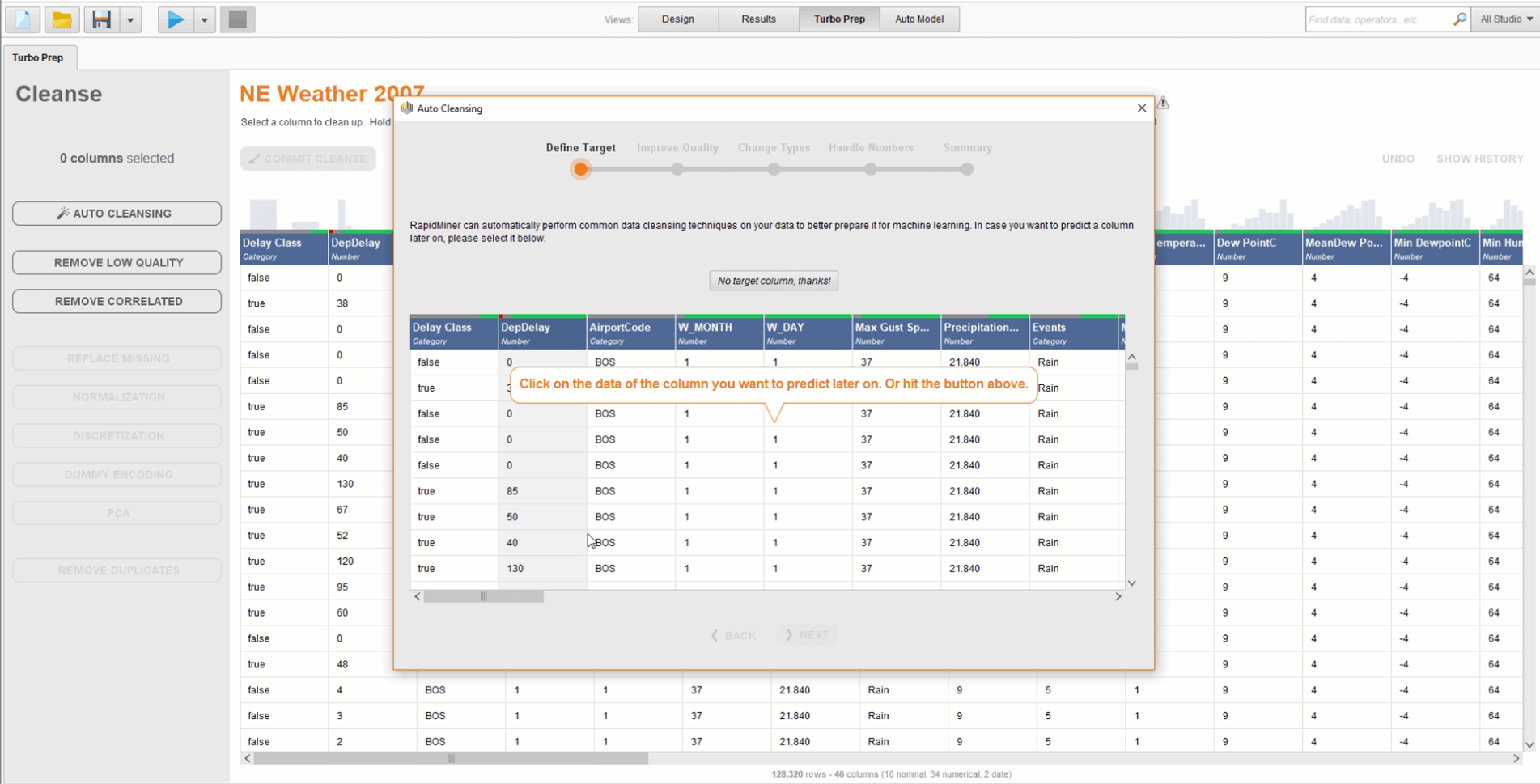
The last step before Modeling, here, is cleansing our data. When we first saw our data, we could see a couple of data quality issues indicated, for example, in the ‘Cancellation’ column, so we know that needs to be addressed. We could go through the data column by column, or we could use the ‘Auto Cleansing’ feature. Clicking on that feature will pop up a dialogue box, prompting us to identify what we would like to predict.
RapidMiner Turbo Prep auto cleansing option
Defining a target in auto cleanse
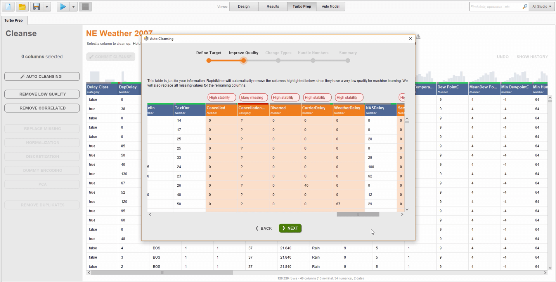
Based on that selection, RapidMiner suggests and selects the columns that should be removed. These are suggested because there is too much data missing or because the data is too stable, for example. By simply clicking ‘Next’ those columns are removed. There are more ways to improve the data quality, but that step is the only one we will use for this example, leaving the rest to the default settings. Then, we click ‘Commit Cleanse’.
Removing columns with quality issues in auto cleanse
Viewing the Process
History
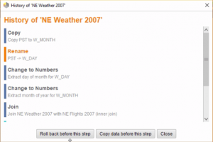
We made quite a few changes and we can review them all by clicking on ‘History’, which shows all of the individual steps we took. If we want to, we can click on one of the steps and decide to roll back the changes before that step or create a copy of the rollback step.
History view
RapidMiner Studio process
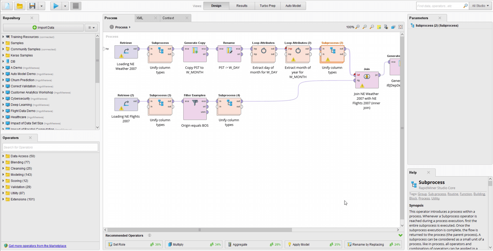
Possibly the most exciting aspect of Turbo Prep is that we can see the full data preparation process by clicking ‘Process’, leading to a fully annotated view in RapidMiner Studio. There are no black boxes in RapidMiner. We can see every step and can make edits and changes as necessary. Whenever we see a model that we like, we can click on it and can open the process. The process is generated with annotations, so we get a full explanation of what happens. We can save this, we can apply it on new data sets, say the flight data from 2008, and we can share this process with our colleagues, or we can deploy it and run it frequently.
Process view in RapidMiner Studio
The results can also be exported into the RapidMiner repositories, into various file formats, or it can be handed over to RapidMiner Auto Model for immediate model creation. In this case, we are going to explore building some quick models using RapidMiner Auto Model by simply clicking on the ‘Auto Model’ tab.
Predicting Delays using Automated Machine Learning
RapidMiner Auto Model
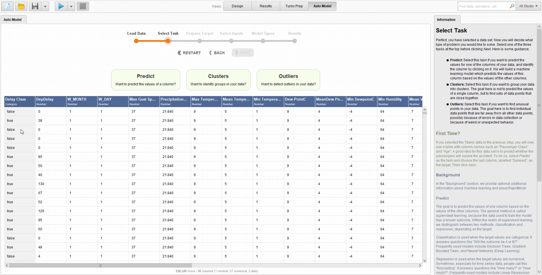
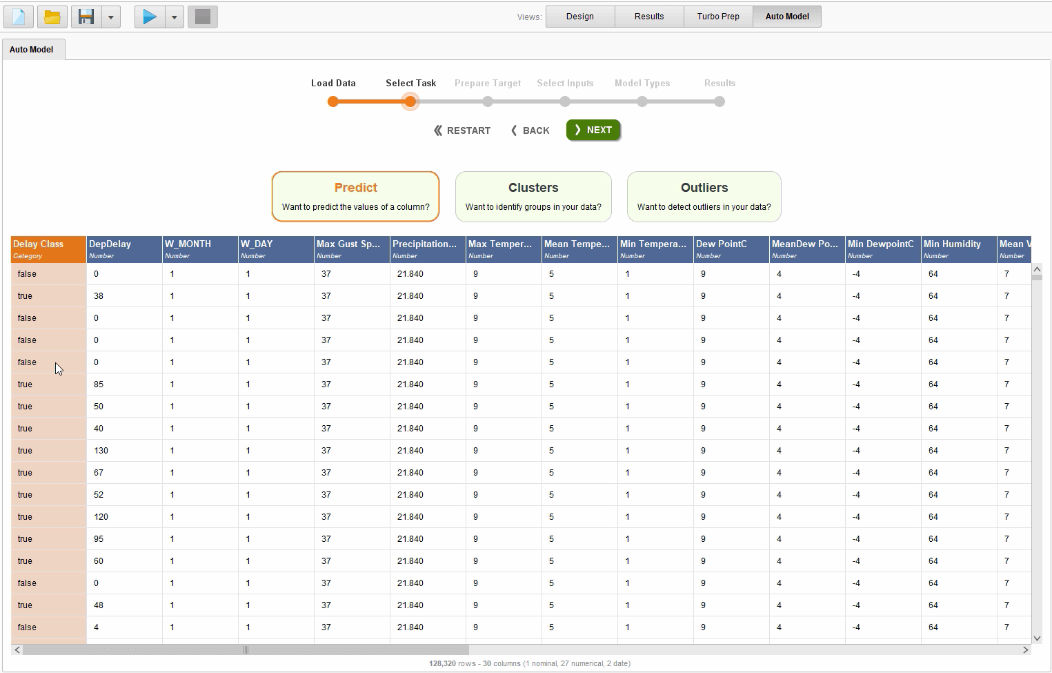
From here, we are able to build some clustering, segmentation, or outlier predictions. In this case, we want to predict the ‘Delay Class’ column. To do that, we just click on the ‘Delay Class’ and ‘Predict’ is already selected so we continue on and click ‘Next’.
Predicting the ‘Delay Class’
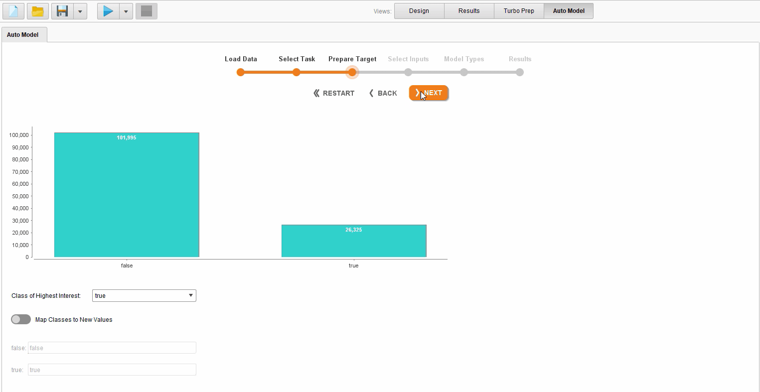
In the ‘Prepare Target’ view, we can choose to map values or change the class of highest interest, but we are most interested in predicting delays, so we will keep the default settings here.
Prepare target view in RapidMiner Auto Model
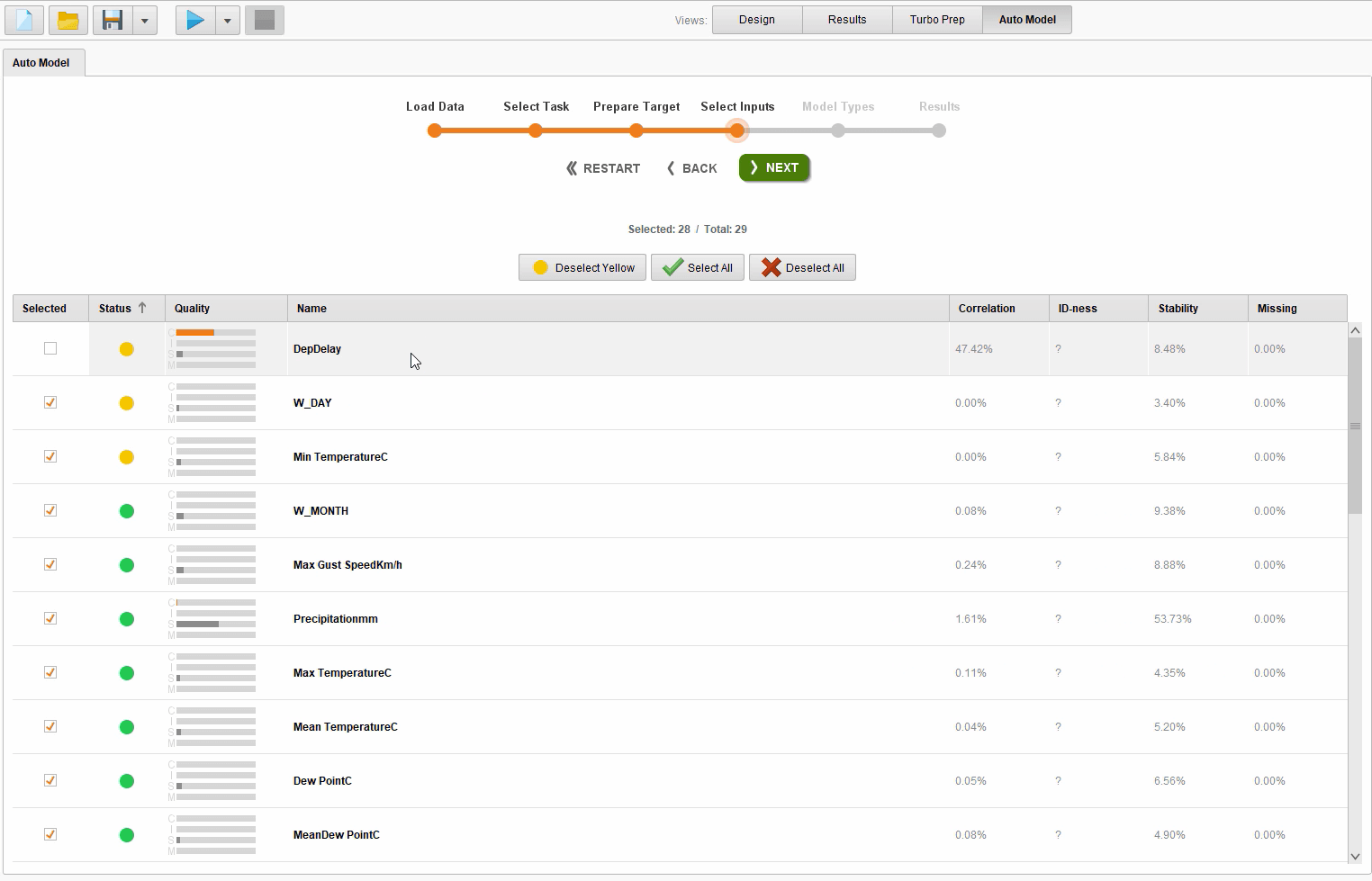
On the next screen, we see those quality measurements are visible again, and we see that there are no red columns in this overview. That’s because we did the auto cleansing already in Turbo Prep. But we do still have a couple of suspicious columns marked in yellow. It is important that Auto Model is pointing out the ‘DepDelay’ as a suspicious column because this is the column that we used to create our predictions. If you recall, when the ‘DepDelay’ is greater than 15 minutes late then this is a delay, otherwise, it is not. If we kept this in, all of the models would focus on that one column and that is not what we want to base our predictions on, so we have to remove the column. In this case, we are also going to remove the other two suspicious columns by clicking ‘Deselect Yellow’ but those could stay in. This is an important feature of Turbo Prep and Auto Model, while we automate as much as we can, we still give the option to overwrite the recommendations.
Removing suspicious columns in yellow
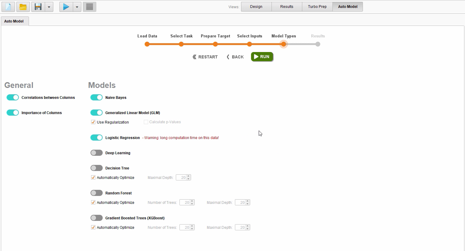
With all three suspicious columns deselected, we click ‘Next’ and move on to the ‘Model Types’ view. In this view, we see a couple of models selected already (suggested by Auto Model), Naïve Bayes and GLM and we can choose to see Logistic Regression as well here.
Selecting the model types
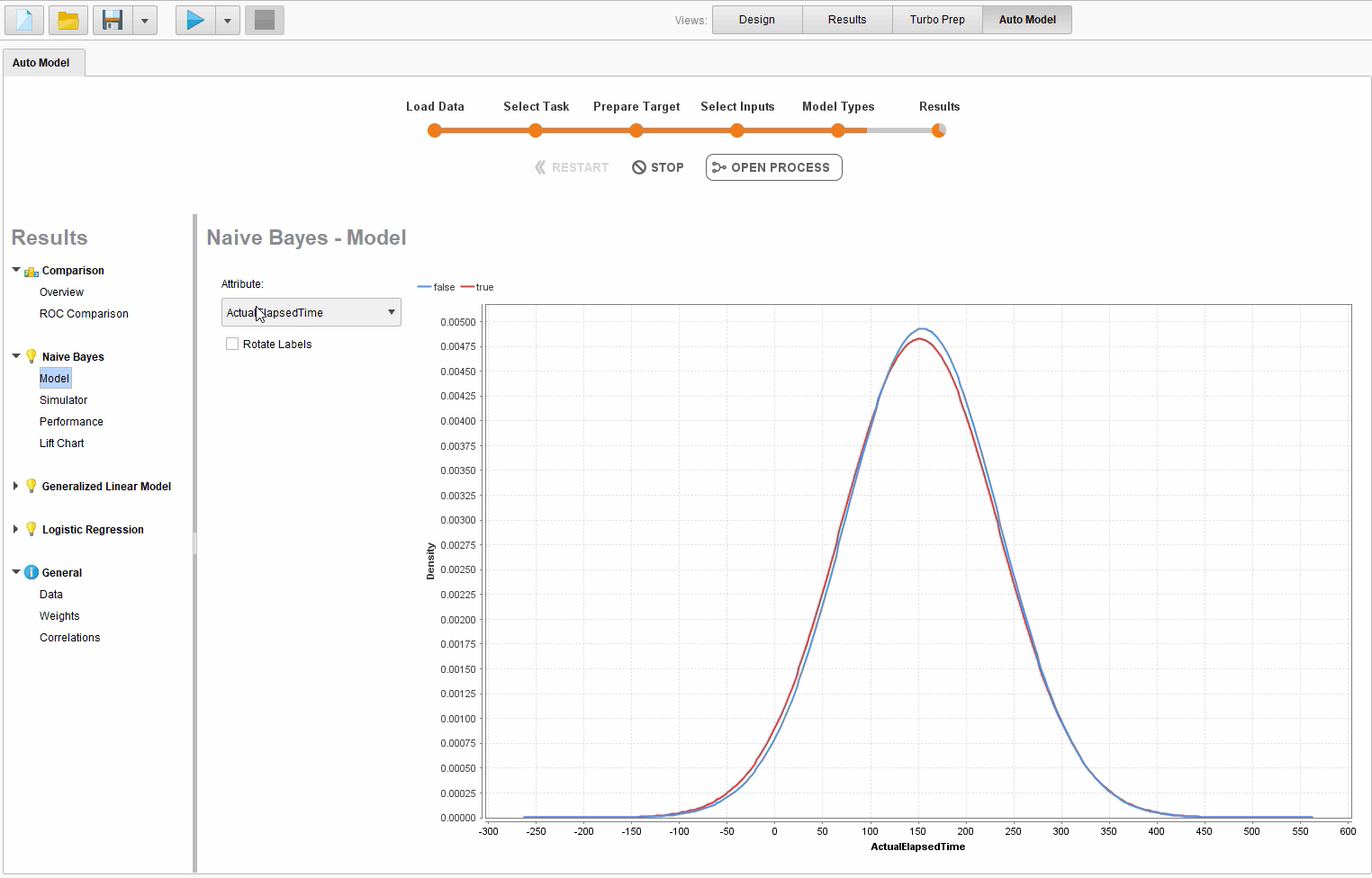
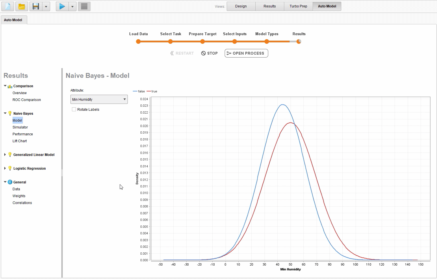
In a few seconds, we see the Naïve Bayes model and can start inspecting it by clicking on ‘Model’ underneath ‘Naïve Bayes’ in the Results window. Here we have a visual way to inspect the model, so, for example, the ‘ActualLapsedTime’ attribute isn’t super helpful, but we can dropdown and select ‘Min Humidity’ instead and start to see that the two classes differ a bit.
Actual Lapsed Time
Min Humidity
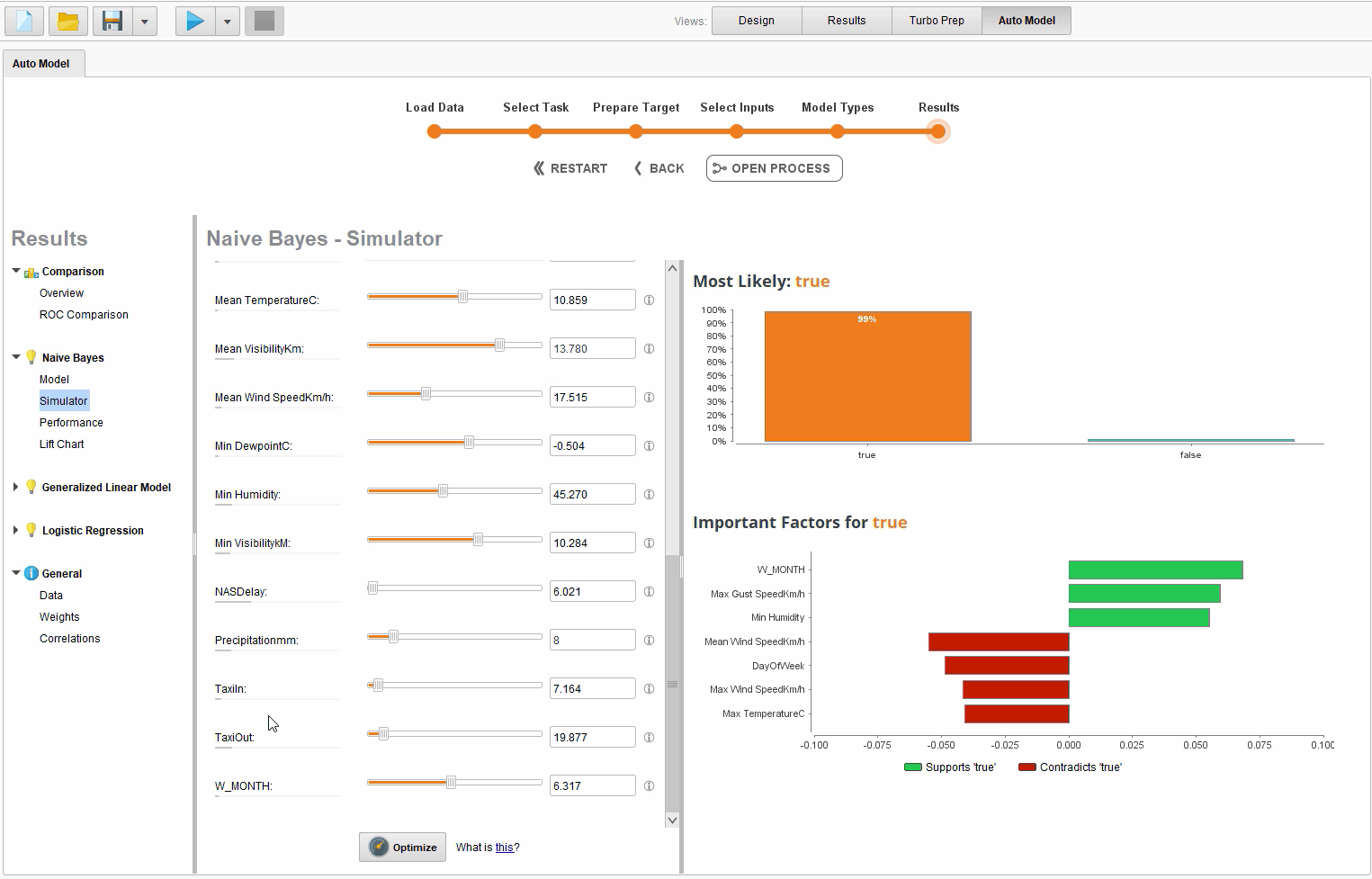
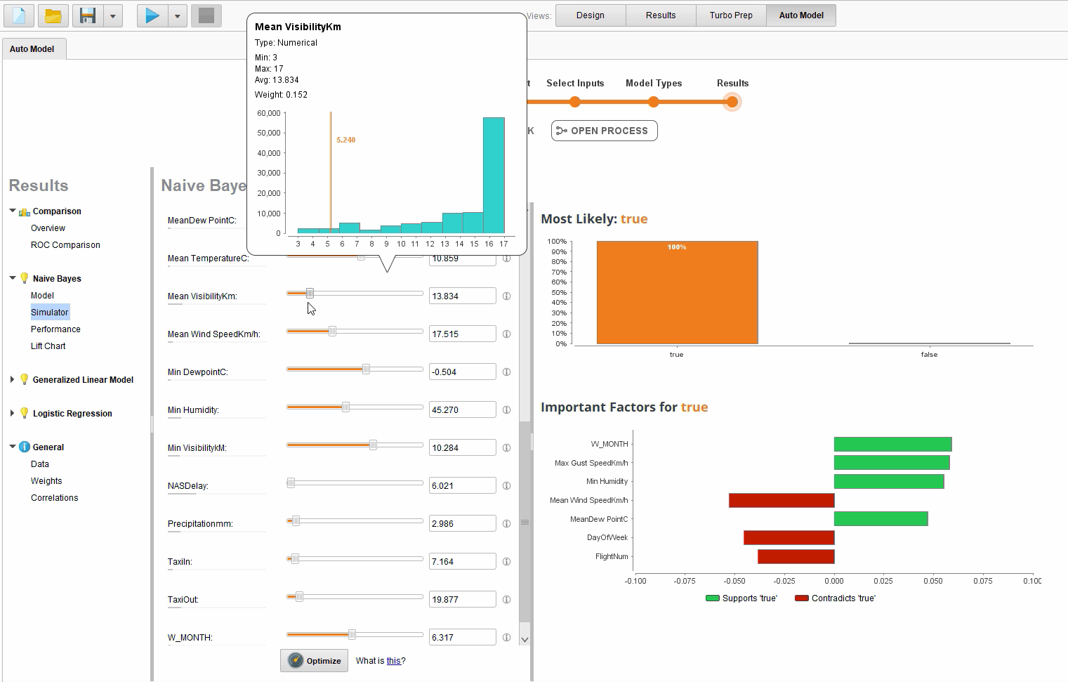
There’s another way to see this information as well, through Auto Model, by clicking on ‘Simulator’ underneath ‘Model’ in the Results window. Here we can experiment with the model a bit. Right off the bat, we see that for the average inputs for our model, it’s more likely that the flight will be delayed. And then we can make some changes. Visibility seems to be pretty important, indicated by the length of the gray bar beneath the class name, so let’s change the visibility a little bit by reducing it, which makes it even more likely that the flight is delayed.
Naïve Bayes simulator with average inputs
Naïve Bayes simulator with decreased visibility
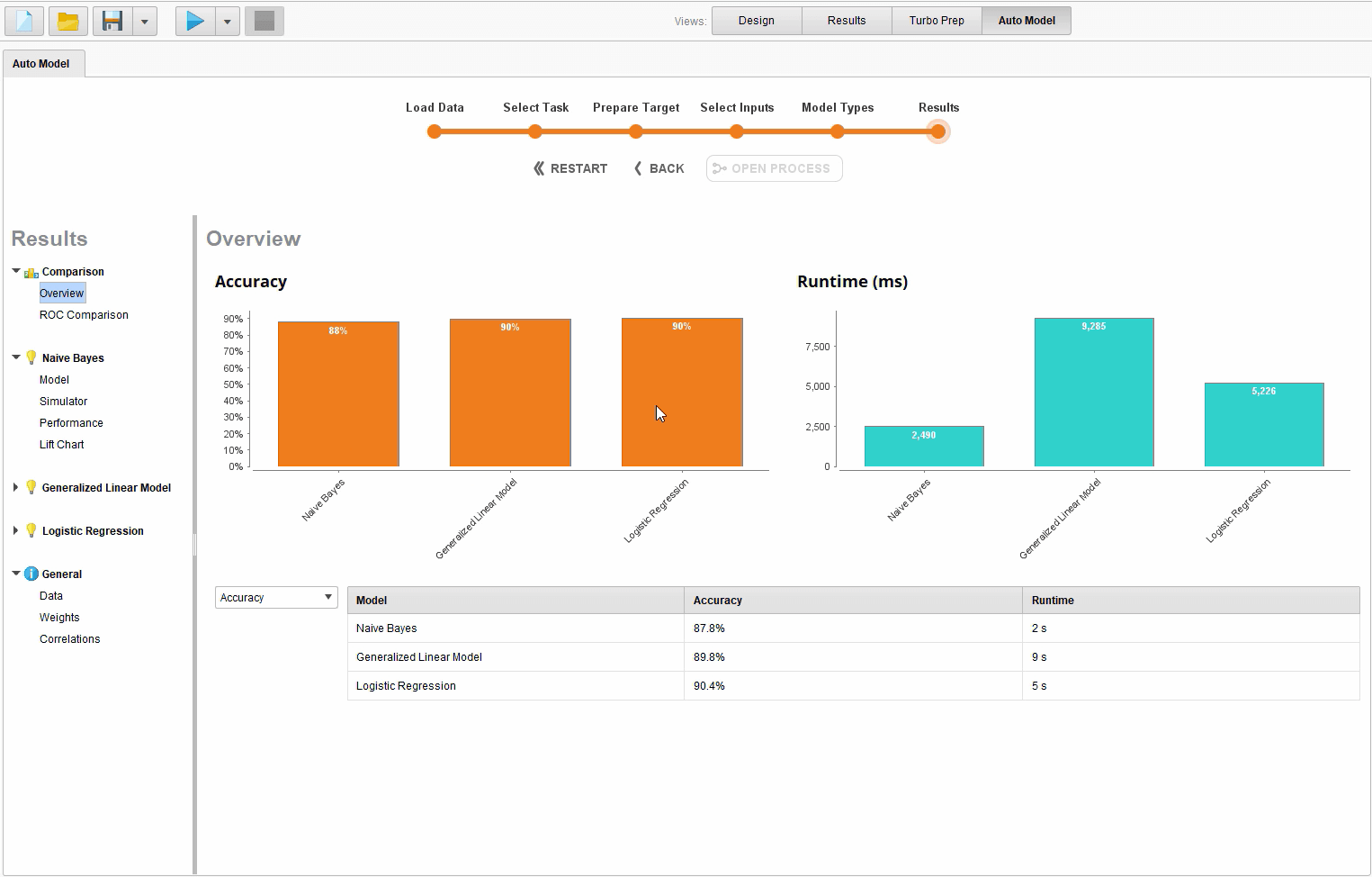
In ‘Overview’ we can see how well the different models performed, here we see that GLM and Logistic Regression performed better than Naïve Bayes. We could also look at the ROC Comparison, or the individual Model Performance and Lift Chart.
Auto Model results overview
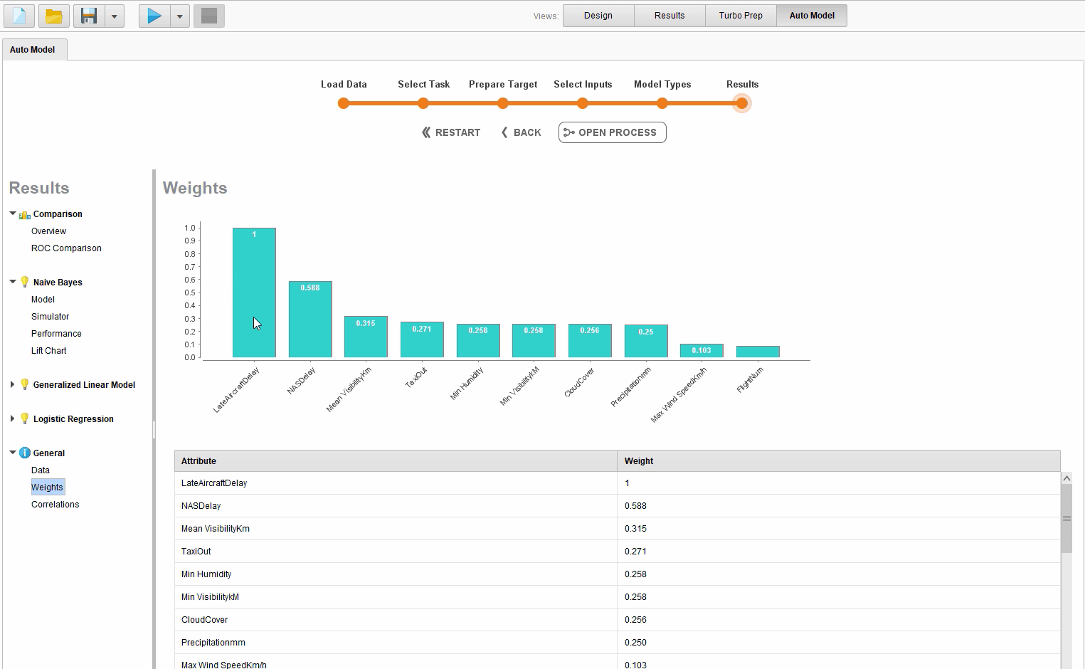
Finally, you can see the data itself, under ‘General’ and the most important influence factors by clicking on ‘Weights’. Here the most influential factor is if the incoming aircraft is delayed, which makes sense. We may want to consider taking that out because it might not be something that we can influence but we will keep it in for now.
Important influence factors
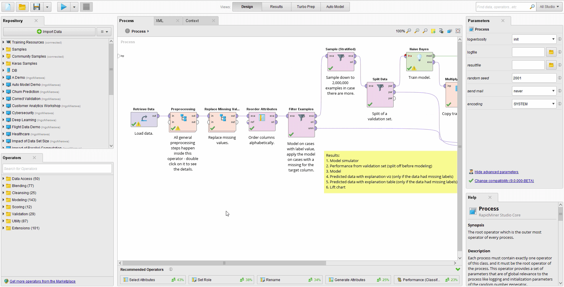
And just like Turbo Prep, Auto Model processes can be opened in RapidMiner Studio, showing the full process with annotations. With Auto Model, every step is explained with its importance and why certain predictions are made during model creation. We can see exactly how the full model was created; there are no black boxes!
Auto Model process
Data Preparation and Machine Learning Simplified
Through this demonstration, we’ve shown that Turbo Prep is an incredibly exciting and useful new capability, radically simplifying and accelerating the time-consuming data preparation task. We demonstrated that it makes it easy to quickly extract, join, filter, group, pivot, transform and cleanse data. You can also connect to a variety of sources like relational databases, spreadsheets, applications, social media, and more.
You can also create repeatable data prep steps, making it faster to reuse processes. Data can also be saved as Excel or CSV or sent to data visualization products like Qlik.
We also demonstrated that once we’re ready to build predictive models with the newly transformed data it’s simple to jump into Auto Model with just one click. RapidMiner Auto Model, unlike any other tool available in the market, automates machine learning by leveraging a decade of data science wisdom so you can focus on quickly unlocking valuable insights from your data. And best of all, there are no black boxes, we can always see exactly what happened in the background and we can replicate it.
If you haven’t tried these two features yet, we’re offering a 30-day trial of Studio Large to all free users so download it now.
About RapidMiner
RapidMiner brings artificial intelligence to the enterprise through an open and extensible data science platform. Built for analytics teams, RapidMiner unifies the entire data science lifecycle from data prep to machine learning to predictive model deployment. 400,000 analytics professionals use RapidMiner products to drive revenue, reduce costs, and avoid risks. For more information visit www.rapidminer.com.
This sponsored post has been written by RapidMiner and all opinions expressed in this post are entirely those of RapidMiner.


