Introduction
What’s the first thing that comes to your mind when you hear the words “reinforcement learning”? The most common thought is – too complex with way too much math. But I’m here to assure you that this is quite a fascinating field of study – and I aim to break down these techniques in my articles into easy-to-understand concepts.
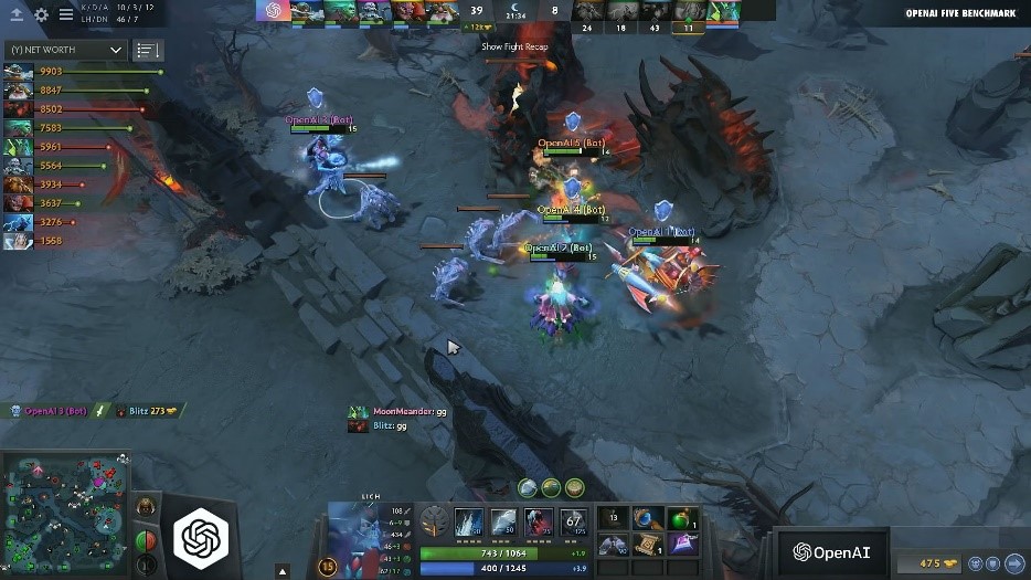
I’m sure you must have heard of OpenAI and DeepMind. These are two leading AI organizations who have made significant progress in this field. A team of OpenAI bots was able to defeat a team of amateur gamers in Dota 2, a phenomenally popular and complex battle arena game.
Do you think it’s feasible to build a bot using dynamic programming for something as complex as Dota 2?
It’s unfortunately a no-go. There are just too many states (millions and millions), and collecting all the specifics of DOTA 2 is an impossible task. This is where we enter the realm of reinforcement learning or more specifically model-free learning.
In this article, we will try to understand the basics of Monte Carlo learning. It’s used when there is no prior information of the environment and all the information is essentially collected by experience. We’ll use the OpenAI Gym toolkit in Python to implement this method as well.
Let’s get the ball rolling!
If you’re a beginner in this field or need a quick refresher of some basic reinforcement learning terminologies, I highly recommend going through the below articles to truly maximize your learning from this post:
- Simple Beginner’s guide to Reinforcement Learning & its implementation
- Nuts & Bolts of Reinforcement Learning: Model Based Planning using Dynamic Programming
- Reinforcement Learning Guide: Solving the Multi-Armed Bandit Problem from Scratch in Python
Table of Contents
- Model-Based vs Model-Free Learning
- Monte Carlo Methods – An Example
- Monte Carlo Reinforcement Learning
- Monte Carlo Prediction
- Monte Carlo Control
- Implementation in Python using OpenAI Gym
Model-Based vs Model-Free Learning
We know that dynamic programming is used to solve problems where the underlying model of the environment is known beforehand (or more precisely, model-based learning). Reinforcement Learning is all about learning from experience in playing games. And yet, in none of the dynamic programming algorithms, did we actually play the game/experience the environment. We had a full model of the environment, which included all the state transition probabilities.
However, in most real life situations as we saw in the introduction, the transition probabilities from one state to another (or the so called model of the environment) are not known beforehand. It is not even necessary that the task follows a Markov property.
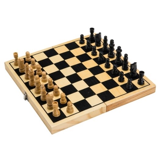
Let’s say we want to train a bot to learn how to play chess. Consider converting the chess environment into an MDP.
Now, depending on the positioning of pieces, this environment will have many states (more than 1050), as well as a large number of possible actions. The model of this environment is almost impossible to design!
One potential solution could be to repeatedly play a complete game of chess and receive a positive reward for winning, and a negative reward for losing, at the end of each game. This is called learning from experience.
Monte Carlo Methods – An Example
Any method which solves a problem by generating suitable random numbers, and observing that fraction of numbers obeying some property or properties, can be classified as a Monte Carlo method.
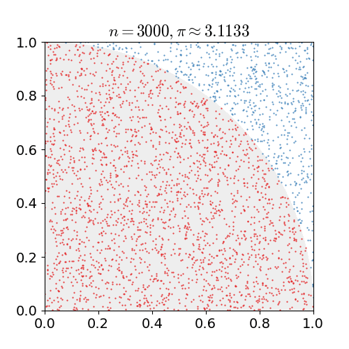
Let’s do a fun exercise where we will try to find out the value of pi using pen and paper. Let’s draw a square of unit length and draw a quarter circle with unit length radius. Now, we have a helper bot C3PO with us. It is tasked with putting as many dots as possible on the square randomly 3,000 times, resulting in the following figure:
C3PO needs to count each time it puts a dot inside a circle. So, the value of pi will be given by:
where N is the number of times a dot was put inside the circle. As you can see, we did not do anything except count the random dots that fall inside the circle and then took a ratio to approximate the value of pi.
Monte Carlo Reinforcement Learning
The Monte Carlo method for reinforcement learning learns directly from episodes of experience without any prior knowledge of MDP transitions. Here, the random component is the return or reward.
One caveat is that it can only be applied to episodic MDPs. Its fair to ask why, at this point. The reason is that the episode has to terminate before we can calculate any returns. Here, we don’t do an update after every action, but rather after every episode. It uses the simplest idea – the value is the mean return of all sample trajectories for each state.
Recalling the idea from multi-armed bandits discussed in this article, every state is a separate multi-armed bandit problem and the idea is to behave optimally for all multi-armed bandits at once.
Similar to dynamic programming, there is a policy evaluation (finding the value function for a given random policy) and policy improvement step (finding the optimum policy). We will cover both these steps in the next two sections.
Monte Carlo Policy Evaluation
The goal here, again, is to learn the value function vpi(s) from episodes of experience under a policy pi. Recall that the return is the total discounted reward:
S1, A1, R2, ….Sk ~ pi
Also recall that the value function is the expected return:
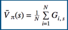
We know that we can estimate any expected value simply by adding up samples and dividing by the total number of samples:
- i – Episode index
- s – Index of state
The question is how do we get these sample returns? For that, we need to play a bunch of episodes and generate them.
For every episode we play, we’ll have a sequence of states and rewards. And from these rewards, we can calculate the return by definition, which is just the sum of all future rewards.
First Visit Monte Carlo: Average returns only for first time s is visited in an episode.
Here’s a step-by-step view of how the algorithm works:
- Initialize the policy, state-value function
- Start by generating an episode according to the current policy
- Keep track of the states encountered through that episode
- Select a state in 2.1
- Add to a list the return received after first occurrence of this state
- Average over all returns
- Set the value of the state as that computed average
- Repeat step 3
- Repeat 2-4 until satisfied
Every visit Monte Carlo: Average returns for every time s is visited in an episode.
For this algorithm, we just change step #3.1 to ‘Add to a list the return received after every occurrence of this state’.
Let’s consider a simple example to further understand this concept. Suppose there’s an environment where we have 2 states – A and B. Let’s say we observed 2 sample episodes:
A+3 => A indicates a transition from state A to state A, with a reward +3. Let’s find out the value function using both methods:
Incremental Mean
It is convenient to convert the mean return into an incremental update so that the mean can be updated with each episode and we can understand the progress made with each episode. We already learnt this when solving the multi-armed bandit problem.
We update v(s) incrementally after episodes. For each state St, with return Gt:
In non-stationary problems, it can be useful to track a running mean, i.e., forget old episodes:
V(St) ← V(St) + α (Gt − V(St))
Monte Carlo Control
Similar to dynamic programming, once we have the value function for a random policy, the important task that still remains is that of finding the optimal policy using Monte Carlo.
Recall that the formula for policy improvement in DP required the model of the environment as shown in the following equation:
This equation finds out the optimal policy by finding actions that maximize the sum of rewards. However, a major caveat here is that it uses transition probabilities, which is not known in the case of model-free learning.
Since we do not know the state transition probabilities p(s’,r/s,a), we can’t do a look-ahead search like DP. Hence, all the information is obtained via experience of playing the game or exploring the environment.
Policy improvement is done by making the policy greedy with respect to the current value function. In this case, we have an action-value function, and therefore no model is needed to construct the greedy policy.
A greedy policy (like the above mentioned one) will always favor a certain action if most actions are not explored properly. There are two solutions for this:
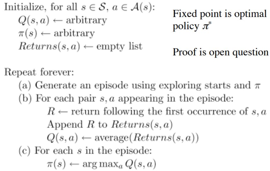
Monte Carlo with exploring starts
All the state action pairs have non-zero probability of being the starting pair, in this algorithm. This will ensure each episode which is played will take the agent to new states and hence, there is more exploration of the environment.
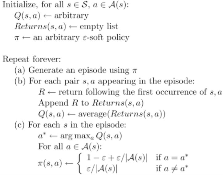
Monte Carlo with epsilon-Soft
What if there is a single start point for an environment (for example, a game of chess)? Exploring starts is not the right option in such cases. Recall here that in a multi-armed bandit problem, we discussed the epsilon-greedy approach.
Simplest idea for ensuring continual exploration all actions are tried with non-zero probability 1 – epsilon choose the action which maximises the action value function and with probability epsilon choose an action at random.
Now that we understand the basics of Monte Carlo Control and Prediction, let’s implement the algorithm in Python. We will import the frozen lake environment from the popular OpenAI Gym toolkit.
Monte Carlo Implementation in Python
Frozen Lake Environment
The agent controls the movement of a character in a grid world. Some tiles of the grid are walkable, and others lead to the agent falling into the water. Additionally, the movement direction of the agent is uncertain and only partially depends on the chosen direction. The agent is rewarded for finding a walkable path to a goal tile.
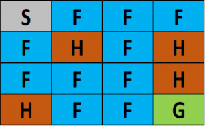
The surface is described using a grid like the following:
(S: starting point, safe), (F: frozen surface, safe), (H: hole, fall to your doom), (G: goal)
The idea is to reach the goal from the starting point by walking only on a frozen surface and avoiding all the holes. Installation details and documentation for the OpenAI Gym are available at this link. Let’s begin!
First, we will define a few helper functions to set up the Monte Carlo algorithm.
Create Environment
Python Code:
Function for Random Policy
def create_random_policy(env):
     policy = {}
     for key in range(0, env.observation_space.n):
          current_end = 0
          p = {}
          for action in range(0, env.action_space.n):
               p[action] = 1 / env.action_space.n
          policy[key] = p
     return policy
Dictionary for storing the state action value
def create_state_action_dictionary(env, policy):
    Q = {}
    for key in policy.keys():
         Q[key] = {a: 0.0 for a in range(0, env.action_space.n)}
    return Q
Function to play episode
def run_game(env, policy, display=True):
     env.reset()
     episode = []
     finished = False

     while not finished:
          s = env.env.s
          if display:
               clear_output(True)
               env.render()
               sleep(1)

          timestep = []
          timestep.append(s)
           n = random.uniform(0, sum(policy[s].values()))
           top_range = 0
           for prob in policy[s].items():
                 top_range += prob[1]
                 if n < top_range:
                       action = prob[0]
                       break
           state, reward, finished, info = env.step(action)
           timestep.append(action)
           timestep.append(reward)

           episode.append(timestep)

     if display:
          clear_output(True)
          env.render()
          sleep(1)
     return episode
Function to test policy and print win percentage
def test_policy(policy, env):
      wins = 0
      r = 100
      for i in range(r):
            w = run_game(env, policy, display=False)[-1][-1]
            if w == 1:
                  wins += 1
      return wins / r
First Visit Monte Carlo Prediction and Control
def monte_carlo_e_soft(env, episodes=100, policy=None, epsilon=0.01):
    if not policy:
        policy = create_random_policy(env)  # Create an empty dictionary to store state action values
    Q = create_state_action_dictionary(env, policy) # Empty dictionary for storing rewards for each state-action pair
    returns = {} # 3.

    for _ in range(episodes): # Looping through episodes
        G = 0 # Store cumulative reward in G (initialized at 0)
        episode = run_game(env=env, policy=policy, display=False) # Store state, action and value respectively

        # for loop through reversed indices of episode array.
        # The logic behind it being reversed is that the eventual reward would be at the end.
        # So we have to go back from the last timestep to the first one propagating result from the future.

        for i in reversed(range(0, len(episode))):
            s_t, a_t, r_t = episode[i]
            state_action = (s_t, a_t)
            G += r_t # Increment total reward by reward on current timestep

            if not state_action in [(x[0], x[1]) for x in episode[0:i]]: #
                if returns.get(state_action):
                    returns[state_action].append(G)
                else:
                    returns[state_action] = [G]

                Q[s_t][a_t] = sum(returns[state_action]) / len(returns[state_action]) # Average reward across episodes

                Q_list = list(map(lambda x: x[1], Q[s_t].items())) # Finding the action with maximum value
                indices = [i for i, x in enumerate(Q_list) if x == max(Q_list)]
                max_Q = random.choice(indices)

                A_star = max_Q # 14.

                for a in policy[s_t].items(): # Update action probability for s_t in policy
                    if a[0] == A_star:
                        policy[s_t][a[0]] = 1 - epsilon + (epsilon / abs(sum(policy[s_t].values())))
                    else:
                        policy[s_t][a[0]] = (epsilon / abs(sum(policy[s_t].values())))

    return policy
Now, it is time to run this algorithm to solve an 8×8 frozen lake environment and check the reward:
On running this for 50,000 episodes, we get a score of 0.9. And with more episodes, it eventually reaches the optimal policy.
End Notes
The story of Monte Carlo learning does not end here. There is another set of algorithms under this which are called off policy Monte Carlo methods. Off policy methods try to learn an optimal policy using returns generated from another policy.
The methods discussed in this article are on policy methods which is basically like learning while doing the job. Whereas off policy methods are akin to learning while watching other people doing the job. I will cover off policy methods in a subsequent article.
If you have any questions or suggestions regarding this article, feel free to connect with me in the comments section below.


