Introduction
Do you have a favorite coffee place in town? When you think of having a coffee, you might just go to this place as you’re almost sure that you will get the best coffee. But this means you’re missing out on the coffee served by this place’s cross-town competitor.
And if you try out all the coffee places one by one, the probability of tasting the worse coffee of your life would be pretty high! But then again, there’s a chance you’ll find an even better coffee brewer. But what does all of this have to do with reinforcement learning?

I’m glad you asked.
The dilemma in our coffee tasting experiment arises from incomplete information. In other words, we need to gather enough information to formulate the best overall strategy and then explore new actions. This will eventually lead to minimizing the overall bad experiences.
A multi-armed bandit is a simplified form of this analogy. It is used to represent similar kinds of problems and finding a good strategy to solve them is already helping a lot of industries.
In this article, we will first understand what actually is a multi-armed bandit problem, it’s various use cases in the real-world, and then explore some strategies on how to solve it. I will then show you how to solve this challenge in Python using a click-through rate optimization dataset.
Table of contents
What is the Multi-Armed Bandit Problem (MABP)?
A bandit is defined as someone who steals your money. A one-armed bandit is a simple slot machine wherein you insert a coin into the machine, pull a lever, and get an immediate reward. But why is it called a bandit? It turns out all casinos configure these slot machines in such a way that all gamblers end up losing money!
A multi-armed bandit is a complicated slot machine wherein instead of 1, there are several levers which a gambler can pull, with each lever giving a different return. The probability distribution for the reward corresponding to each lever is different and is unknown to the gambler.

The task is to identify which lever to pull in order to get maximum reward after a given set of trials. This problem statement is like a single step Markov decision process, which I discussed in this article. Each arm chosen is equivalent to an action, which then leads to an immediate reward.
Exploration Exploitation in the context of Bernoulli MABP
The below table shows the sample results for a 5-armed Bernoulli bandit with arms labelled as 1, 2, 3, 4 and 5:
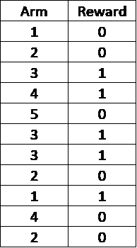
This is called Bernoulli, as the reward returned is either 1 or 0. In this example, it looks like the arm number 3 gives the maximum return and hence one idea is to keep playing this arm in order to obtain the maximum reward (pure exploitation).
Just based on the knowledge from the given sample, 5 might look like a bad arm to play, but we need to keep in mind that we have played this arm only once and maybe we should play it a few more times (exploration) to be more confident. Only then should we decide which arm to play (exploitation).
Use Cases
Bandit algorithms are being used in a lot of research projects in the industry. I have listed some of their use cases in this section.
Clinical Trials
The well being of patients during clinical trials is as important as the actual results of the study. Here, exploration is equivalent to identifying the best treatment, and exploitation is treating patients as effectively as possible during the trial.

Network Routing
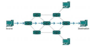
Routing is the process of selecting a path for traffic in a network, such as telephone networks or computer networks (internet). Allocation of channels to the right users, such that the overall throughput is maximised, can be formulated as a MABP.
Online Advertising
The goal of an advertising campaign is to maximise revenue from displaying ads. The advertiser makes revenue every time an offer is clicked by a web user. Similar to MABP, there is a trade-off between exploration, where the goal is to collect information on an ad’s performance using click-through rates, and exploitation, where we stick with the ad that has performed the best so far.

Game Designing
Building a hit game is challenging. MABP can be used to test experimental changes in game play/interface and exploit the changes which show positive experiences for players.

Solution Strategies
In this section, we will discuss some strategies to solve a multi-armed bandit problem. But before that, let’s get familiar with a few terms we’ll be using from here on.
Action-Value Function
The expected payoff or expected reward can also be called an action-value function. It is represented by q(a) and defines the average reward for each action at a time t.

Suppose the reward probabilities for a K-armed bandit are given by {P1, P2, P3 …… Pk}. If the ith arm is selected at time t, then Qt(a) = Pi.
The question is, how do we decide whether a given strategy is better than the rest? One direct way is to compare the total or average reward which we get for each strategy after n trials. If we already know the best action for the given bandit problem, then an interesting way to look at this is the concept of regret.
Regret
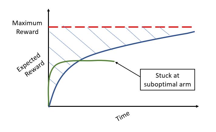
Let’s say that we are already aware of the best arm to pull for the given bandit problem. If we keep pulling this arm repeatedly, we will get a maximum expected reward which can be represented as a horizontal line (as shown in the figure below):
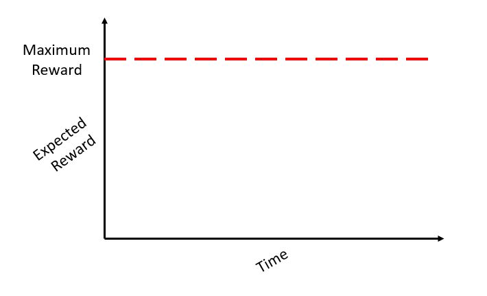
But in a real problem statement, we need to make repeated trials by pulling different arms till we am approximately sure of the arm to pull for maximum average return at a time t. The loss that we incur due to time/rounds spent due to the learning is called regret. In other words, we want to maximise my reward even during the learning phase. Regret is very aptly named, as it quantifies exactly how much you regret not picking the optimal arm.
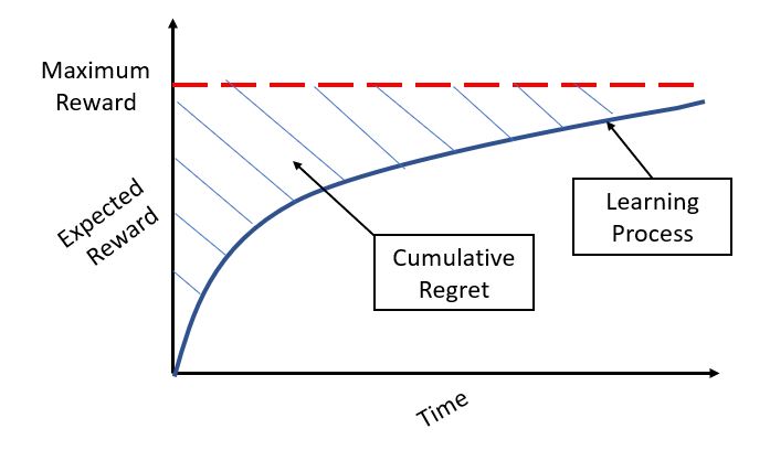
Now, one might be curious as to how does the regret change if we are following an approach that does not do enough exploration and ends exploiting a suboptimal arm. Initially there might be low regret but overall we are far lower than the maximum achievable reward for the given problem as shown by the green curve in the following figure.
Based on how exploration is done, there are several ways to solve the MABP. Next, we will discuss some possible solution strategies.
No Exploration (Greedy Approach)
A naïve approach could be to calculate the q, or action value function, for all arms at each timestep. From that point onwards, select an action which gives the maximum q. The action values for each action will be stored at each timestep by the following function:

It then chooses the action at each timestep that maximises the above expression, given by:

However, for evaluating this expression at each time t, we will need to do calculations over the whole history of rewards. We can avoid this by doing a running sum. So, at each time t, the q-value for each action can be calculated using the reward:

The problem here is this approach only exploits, as it always picks the same action without worrying about exploring other actions that might return a better reward. Some exploration is necessary to actually find an optimal arm, otherwise we might end up pulling a suboptimal arm forever.
Epsilon Greedy Approach
One potential solution could be to now, and we can then explore new actions so that we ensure we are not missing out on a better choice of arm. With epsilon probability, we will choose a random action (exploration) and choose an action with maximum qt(a) with probability 1-epsilon.
With probability 1- epsilon – we choose action with maximum value (argmaxa Qt(a))
With probability epsilon – we randomly choose an action from a set of all actions A
For example, if we have a problem with two actions – A and B, the epsilon greedy algorithm works as shown below:
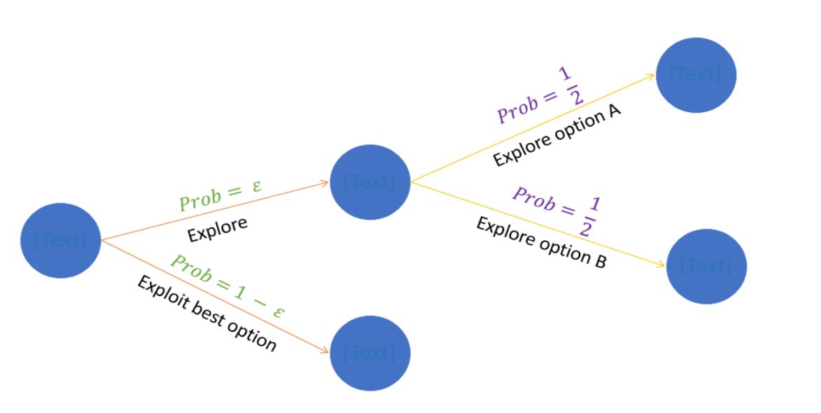
This is much better than the greedy approach as we have an element of exploration here. However, if two actions have a very minute difference between their q values, then even this algorithm will choose only that action which has a probability higher than the others.
Softmax Exploration
The solution is to make the probability of choosing an action proportional to q. This can be done using the softmax function, where the probability of choosing action a at each step is given by the following expression:

Decayed Epsilon Greedy
The value of epsilon is very important in deciding how well the epsilon greedy works for a given problem. We can avoid setting this value by keeping epsilon dependent on time. For example, epsilon can be kept equal to 1/log(t+0.00001). It will keep reducing as time passes, to the point where we starting exploring less and less as we become more confident of the optimal action or arm.
The problem with random selection of actions is that after sufficient timesteps even if we know that some arm is bad, this algorithm will keep choosing that with probability epsilon/n. Essentially, we are exploring a bad action which does not sound very efficient. The approach to get around this could be to favour exploration of arms with a strong potential in order to get an optimal value.
Upper Confidence Bound
Upper Confidence Bound (UCB) is the most widely used solution method for multi-armed bandit problems. This algorithm is based on the principle of optimism in the face of uncertainty.
In other words, the more uncertain we are about an arm, the more important it becomes to explore that arm.
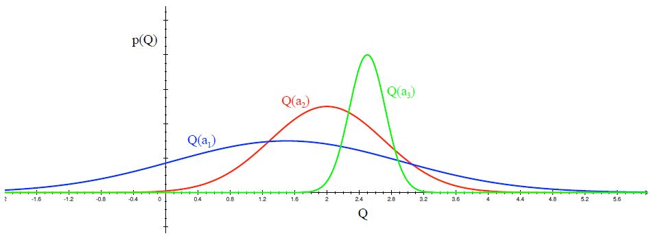
- Distribution of action-value functions for 3 different arms a1, a2 and a3 after several trials is shown in the figure above. This distribution shows that the action value for a1 has the highest variance and hence maximum uncertainty.
- UCB says that we should choose the arm a1 and receive a reward making us less uncertain about its action-value. For the next trial/timestep, if we still are very uncertain about a1, we will choose it again until the uncertainty is reduced below a threshold.
The intuitive reason this works is that when acting optimistically in this way, one of two things happen:
- optimism is justified and we get a positive reward which is the objective ultimately
- the optimism was not justified. In this case, we play an arm that we believed might give a large reward when in fact it does not. If this happens sufficiently often, then we will learn what is the true payoff of this action and not choose it in the future.
UCB is actually a family of algorithms. Here, we will discuss UCB1.
Steps involved in UCB1:
- Play each of the K actions once, giving initial values for mean rewards corresponding to each action at
- For each round t = K:
- Let Nt(a) represent the number of times action a was played so far
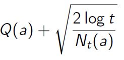
- Play the action at maximising the following expression:
- Observe the reward and update the mean reward or expected payoff for the chosen action
We will not go into the mathematical proof for UCB. However, it is important to understand the expression that corresponds to our selected action. Remember, in the random exploration we just had Q(a) to maximise, while here we have two terms. First is the action value function, while the second is the confidence term.
- Each time a is selected, the uncertainty is presumably reduced: Nt(a) increments, and, as it appears in the denominator, the uncertainty term decreases.
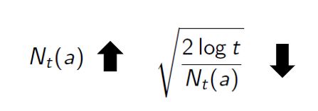
- On the other hand, each time an action other than a is selected, t increases, but Nt(a) does not; because t appears in the numerator, the uncertainty estimate increases.

- The use of the natural logarithm means that the increases get smaller over time; all actions will eventually be selected, but actions with lower value estimates, or that have already been selected frequently, will be selected with decreasing frequency over time.
- This will ultimately lead to the optimal action being selected repeatedly in the end.
Regret Comparison
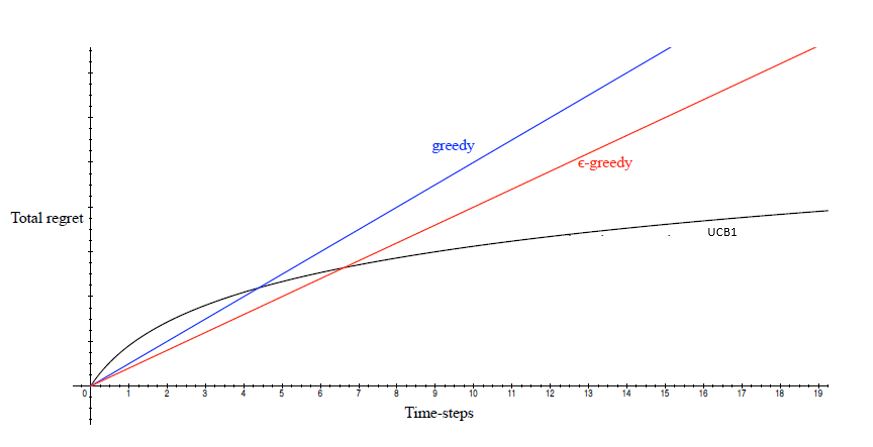
Among all the algorithms given in this article, only the UCB algorithm provides a strategy where the regret increases as log(t), while in the other algorithms we get linear regret with different slopes.
Non-Stationary Bandit problems
An important assumption we are making here is that we are working with the same bandit and distributions from which rewards are being sampled at each timestep stays the same. This is called a stationary problem. To explain it with another example, say you get a reward of 1 every time a coin is tossed, and the result is head. Say after 1000 coin tosses due to wear and tear the coin becomes biased then this will become a non-stationary problem.
To solve a non-stationary problem, more recent samples will be important and hence we could use a constant discounting factor alpha and we can rewrite the update equation like this:

Note that we have replaced Nt(at) here with a constant alpha, which ensures that the recent samples are given higher weights, and increments are decided more by such recent samples. There are other techniques which provide different solutions to bandits with non-stationary rewards. You can read more about them in this paper.
Python Implementation from scratch for Ad CTR Optimization
As mentioned in the use cases section, MABP has a lot of applications in the online advertising domain.
Suppose an advertising company is running 10 different ads targeted towards a similar set of population on a webpage. We have results for which ads were clicked by a user here. Each column index represents a different ad. We have a 1 if the ad was clicked by a user, and 0 if it was not. A sample from the original dataset is shown below:
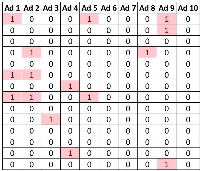
This is a simulated dataset and it has Ad #5 as the one which gives the maximum reward.
First, we will try a random selection technique, where we randomly select any ad and show it to the user. If the user clicks the ad, we get paid and if not, there is no profit.
# Random Selection

# Importing the libraries
import numpy as np
import matplotlib.pyplot as plt
import pandas as pd

# Importing the dataset
dataset = pd.read_csv('Ads_Optimisation.csv')

# Implementing Random Selection
import random
N = 10000
d = 10
ads_selected = []
total_reward = 0
for n in range(0, N):
    ad = random.randrange(d)
    ads_selected.append(ad)
    reward = dataset.values[n, ad]
    total_reward = total_reward + reward
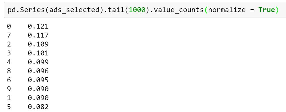
Total reward for the random selection algorithm comes out to be 1170. As this algorithm is not learning anything, it will not smartly select any ad which is giving the maximum return. And hence even if we look at the last 1000 trials, it is not able to find the optimal ad.
Now, let’s try the Upper Confidence Bound algorithm to do the same:
# Implementing UCB
import math
N = 10000
d = 10
ads_selected = []
numbers_of_selections = [0] * d
sums_of_reward = [0] * d
total_reward = 0

for n in range(0, N):
    ad = 0
    max_upper_bound = 0
    for i in range(0, d):
        if (numbers_of_selections[i] > 0):
            average_reward = sums_of_reward[i] / numbers_of_selections[i]
            delta_i = math.sqrt(2 * math.log(n+1) / numbers_of_selections[i])
            upper_bound = average_reward + delta_i
        else:
            upper_bound = 1e400
        if upper_bound > max_upper_bound:
            max_upper_bound = upper_bound
            ad = i
    ads_selected.append(ad)
    numbers_of_selections[ad] += 1
    reward = dataset.values[n, ad]
    sums_of_reward[ad] += reward
    total_reward += reward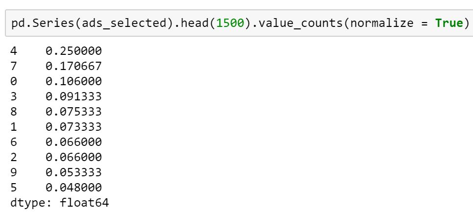
The total_reward for UCB comes out to be 2125. Clearly, this is much better than random selection and indeed a smart exploration technique that can significantly improve our strategy to solve a MABP.
After just 1500 trials, UCB is already favouring Ad #5 (index 4) which happens to be the optimal ad, and gets the maximum return for the given problem.
End Notes
Being an active area of research MABP will percolate to various other fields in the industry. These algorithms are so simple and powerful that they are being used increasingly by even small tech companies, as the computation resources required for them are often low.
Going forward, there are other techniques based on probabilistic models such as Thompson Sampling explained by Professor Balaraman in this amazing video.
You can attend a highly anticipated and extremely useful talk on reinforcement learning from him at DataHack Summit 2018 in Bangalore as well! For more details, please visit https://www.geeksforgeeks.org/datahack-summit-2018/.


