This article was published as a part of the Data Science Blogathon.
Introduction
When training a machine learning model, the model can be easily overfitted or under fitted. To avoid this, we use regularization in machine learning to properly fit the model to our test set. Regularization techniques help reduce the possibility of overfitting and help us obtain an optimal model. In this article titled ‘The Ultimate Guide to Regularization in Machine Learning, you will learn everything you need to know about regularization.
Understanding Overfitting and Underfitting
To train our machine learning model, we provide it with data to learn from. The process of plotting a series of data points and drawing a line of best fit to understand the relationship between variables is called Data Fitting. Our model is best suited when it can find all the necessary patterns in our data and avoid random data points, and unnecessary patterns called noise.
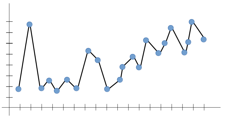
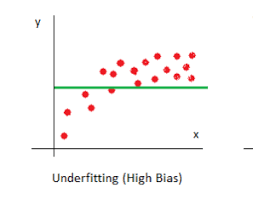
What are the Bias and Variance?
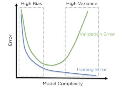
The above figure shows that when the bias is high, the error in both the test and training sets is also high. When the deviation is high, the model performs well on our training set and gives a low error, but the error on our test set is very high. In the middle of this, there is a region where bias and variance are in perfect balance with each other here too, but training and testing errors are low.
Regularization in Machine Learning?
Regularization refers to techniques used to calibrate machine learning models to minimize the adjusted loss function and avoid overfitting or underfitting.

Regularization Techniques
Ridge Regularization
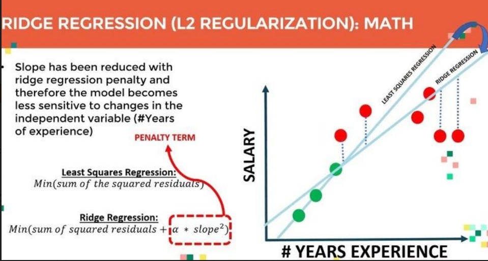
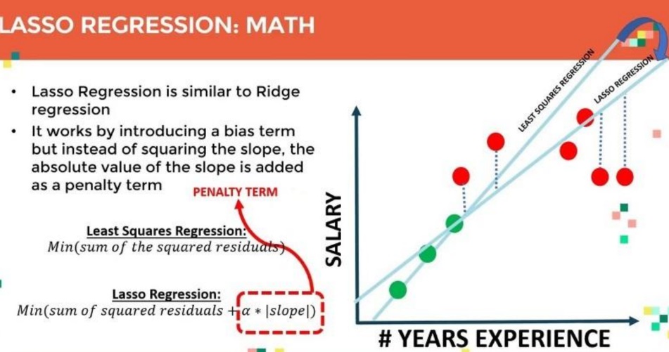
Lasso Regularization
Elastic Net
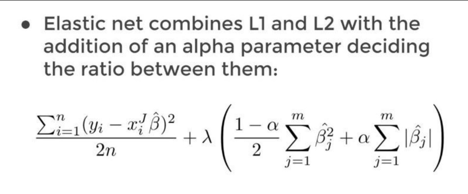
Elastic Net combines L1 and L2 With the addition of an alpha Parameter.
Regularization Using Python in Machine Learning
import numpy as np
import pandas as pd
import matplotlib.pyplot as plt
%matplotlib inline
import seaborn as sns
We then load the Advertisement Dataset from sklearn’s datasets.
df = pd.read_csv("Advertising.csv")
Splitting the Dataset into Training and Testing Dataset:
Applying the Train Train Split:
Python Code:
Now we can use them for training our linear regression model. We’ll start by creating our model and fitting the data into it. We then predict on the test set and find the error in our prediction using mean_squared_error. Finally, we print the coefficients of our linear regression model.
Ridge Regression:
Modelling with default Parameters:
from sklearn.linear_model import Ridge
ridge_model = Ridge()
ridge_model.fit(X_train, y_train)
Predictions and Evaluation Of Ridge Regression:
test_predictions = ridge_model.predict(X_test)
train_predictions = ridge_model.predict(X_train)
Hyperparameter Tuning of Ridge : Identifying the best alpha value for Ridge Regression:
from sklearn.model_selection import GridSearchCV
estimator = Ridge()
estimator = Ridge()
param_grid = {"alpha":list(range(1,11))}
model_hp = GridSearchCV(estimator, param_grid, cv = 5)
model_hp.fit(X_train, y_train)
model_hp.best_params_
Lasso Regularization:
Modeling of Lasso Regularization:
from sklearn.linear_model import Lasso
lasso_model = Lasso()
lasso_model.fit(X_train, y_train)
Predictions and Evaluation Of Lasso Regression:
test_predictions = lasso_model.predict(X_test)
train_predictions = lasso_model.predict(X_train)
from sklearn.metrics import mean_squared_error
train_rmse = np.sqrt(mean_squared_error(y_test, test_predictions))
test_rmse = np.sqrt(mean_squared_error(y_train, train_predictions))
print("train RMSE:", train_rmse)
print("test RMSE:", test_rmse)
Hyperparameter Tuning of Lasso:
Identifying the best alpha value for Lasso Regression:
param_grid = {"alpha": list(range(1,11))}
model_hp = GridSearchCV(estimator, param_grid, cv =5)
model_hp.fit(X_train, y_train)
model_hp.best_estimator_
Elastic Net Regularization:
modeling of Elastic Net Regularization:
from sklearn.linear_model import ElasticNet
enr_model = ElasticNet(alpha=2, l1_ratio = 1)
enr_model.fit(X_train, y_train)
Predictions and Evaluation Of Elastic Net:
test_predictions = enr_model.predict(X_test)
train_predictions = enr_model.predict(X_train)
from sklearn.metrics import mean_squared_error
train_rmse = np.sqrt(mean_squared_error(y_test, test_predictions))
test_rmse = np.sqrt(mean_squared_error(y_train, train_predictions))
print("train RMSE:", train_rmse)
print("test RMSE:", test_rmse)
Hyperparameter Tuning of Elastic Net: Identifying the best alpha value for Elastic Net:
from sklearn.model_selection import GridSearchCV
enr_hp = GridSearchCV(estimator, param_grid)
enr_hp.fit(X_train, y_train)
enr_hp.best_params_
param_grid = { "alpha" : [0, 0.1, 0.2, 1, 2, 3, 5, 10],
"l1_ratio" : [0.1, 0.5, 0.75, 0.9, 0.95, 1]}
estimator = ElasticNet()
Conclusion
Also In this article, we studied Overfittings and Underfitting of a Linear model and how regularization Techniques can be used to overcome these issues.
- We learned about the L1 and L2 Regularization, which are added to the cost function.
- In each of these algorithms, we can set to specify several hyperparameters.
- We can use GridSearchCV or the respective Hyperparameter Tuning algorithms of the given respective regression model to find the optimal hyperparameters.
You can try to compare the performance of these algorithms on a dataset and check which algorithm performed better using a performance metric like Root Mean Square Error or RMSE.
Thank you for reading.
I hope you enjoyed the questions and were able to test your knowledge about Data Science and Machine Learning.
Please feel free to contact me on Linkedin.
email: [email protected]
The media shown in this article is not owned by Analytics Vidhya and is used at the Author’s discretion.


