This article was published as a part of the Data Science Blogathon.
Introduction
In this article, I am trying to showcase my understanding of the Variable Clustering algorithm (the most popular technique for dimension reduction).
Disclaimer: This article aims to share my knowledge of Variable Clustering. This does not include any project-related data, codes, and so on. SAS/Python codes used in this article are purely based on publically available datasets and not relate to any company project. The reader of this article must have a background in Statistics, SAS, and Python.
The complexity of a dataset increases rapidly with increasing dimensionality. It increases the computation time, affects the ability to explore the model relationship, model scoring, increases the redundancy in the dataset, and so on.
One of the remedial measures can be Variable Clustering. It finds a group of variables that are as correlated as possible among themselves within a cluster and as uncorrelated as possible with variables in other clusters.
We will understand the Variable Clustering in below three steps:
1. Principal Component Analysis (PCA)
2. Eigenvalues and Communalities
3. 1 – R_Square Ratio
At the end of these three steps, we will implement the Variable Clustering using SAS and Python in high dimensional data space.
1. PCA — Principal Component Analysis
PCA is the heart of the algorithm. Let us understand how it works. Suppose, we have 10 variables and their correlation among themselves are as follow:
Now, we will create a coefficient for the first principal component or factor. The principal component is the weighted linear combination of predictor variables. It is calculated as follow:
Let me expand the formulas. It is taking column total and row total and then First PC = column_total / sqrt(row_total)
Now, obtain the matrix of residual coefficients (R1) by Table 7 values to Table 2 (R) values.
Now, on this residual matrix, we will perform the same calculations to get the second PC2.
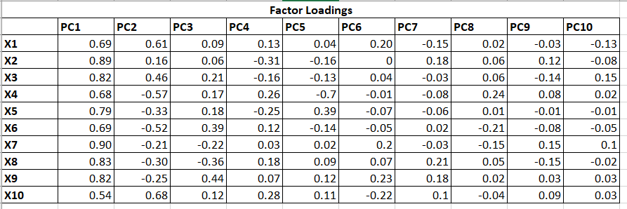
The same process will follow for all the factors/PCs. As we have 10 variables so there will be 10 PCs calculated. Till now, we get the coefficients of PCs as follow:
Table 12 represents the Factor Loadings which are the correlation between each PCs and Variables. If we simply square the values, we will get R2 as follow:
2. Eigenvalue and Communalities:
We can calculate different measures by using Table 13.
Eigenvalue: Variance explained by each PC for all the variables (Column total of each PC).
Communalities: Variance explained by all the PC for a single variable (Row total). It will always sum to 1 as 100% variance explained by all the PCs for a single variable.
Ideally, the first few PCs (say the first two PC in this example)will be retained as they explained most of the variations in the data. And this reduced set of PCs will be used to create scores and that score will be used in place of the original 10 variables.
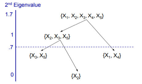
Ok. Now, we are clear about PC, Eigenvalues, Communality, and so on. Variable Clustering uses the same algorithm but instead of using the PC score, we will pick one variable from each Cluster. All the variables start in one cluster. A principal component is done on the variables in the cluster. If the Second Eigenvalue of PC is greater than the specified threshold, then the cluster is split.
3. 1 – R_Square Ratio
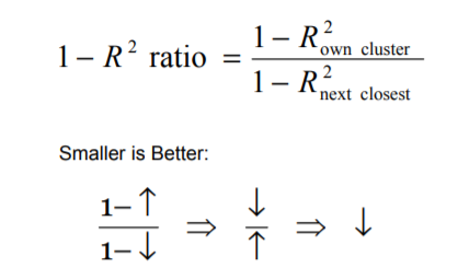
The question is which variable to pick from each cluster? One should pick the variable which is having the highest correlation with its own cluster and low with other clusters.
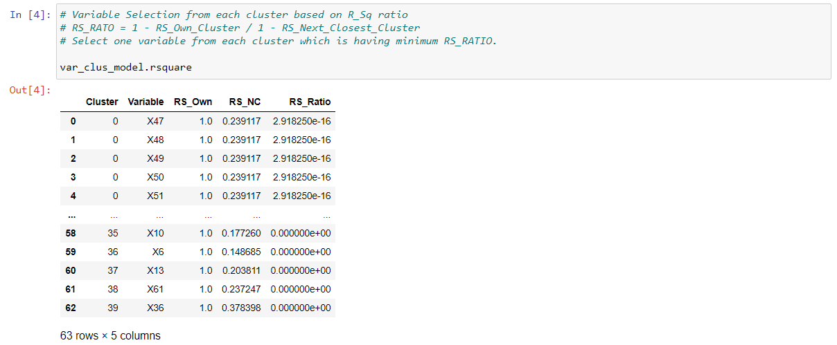
Hence, the variable having the lowest 1 — R2 ratio can be a good representative of the cluster and that variable would be used and other variables from that cluster will be discarded. This is how we can achieve the dimension reduction.
Implementation using SAS and Python:
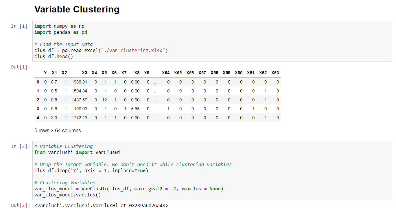
I have a dataset (https://github.com/urvish-stat/Data) containing 63 variables including dummy variables, missing indicator variables, and so on. Not all the variables are important in predictive modeling.
Let’s implement the Variable Clustering to eliminate the redundancy present in the data.
In the last output, it gives us the clusters containing different variables and we will select one variable based on 1-R2_Ratio.
As there are 40 clusters, there will be 40 variables instead of 63 variables.
I used maxeigval = 0.7. It means that clusters will split if the second eigenvalue is greater than 0.7. A larger value of this parameter gives fewer clusters and less of the variations explained. Smaller value gives more clusters and more variation explained. The common choice is 1 as it represents the average size of eigenvalues.
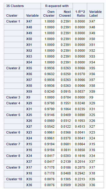
SAS Output for the first 10 clusters:
The total number of Clusters are not matching between SAS and Python. In SAS, there is a total of 35 clusters and in Python, there are 40. However, variable allocations in most of the clusters and their 1 — R2 Ratio are matching.
Thanks,
Urvish Shah


