


This article was published as a part of the Data Science Blogathon.
Introduction
Machine learning is about building a predictive model using historical data to make predictions on new data where you do not have the answer to a particular question. Since, the output is probabilistic, evaluating your predictions becomes a crucial step. There are a lot of ways by which you can judge how well your machine learning model performs and mostly all of them focus on minimizing the error between the actual and predicted entity because you would want your predictions to be more and more accurate.
Supervised learning algorithms, where you have information about the labels like in classification, regression problems, and unsupervised learning algorithms, where you don’t have the label information such as clustering, have different evaluation metrics according to their outputs. In this post, you will explore some of the most popular evaluation metrics for classification, regression, and clustering problems. More specifically, you’ll :
– learn all the terms related to the confusion matrix and metrics drawn from it
– learn evaluation metrics like RMSE, MAE, R-Squared, etc. for regression problems
– learn metrics like Silhouette coefficient, Dunn’s index for clustering problems
All the evaluation metrics described in this tutorial have an implementation available as libraries, packages on different platforms like Python, R, Spark, etc., however, this tutorial is only concerned with the meaning of these metrics which you should be aware of before using them. You can use this guide as a quick reference in case you need to quickly revise the important metrics in machine learning.
Let’s get started.
Classification Performance Evaluation Metrics
Perhaps the most common form of machine learning problems is classification problems. A classification problem puts an observation/sample into one of two or more classes/labels. Essentially you are trying to learn a mathematical function that can classify your input variables (X) to discrete output variables (Y). The output variables are called classes/labels. For example, classifying an email as spam or not-spam is a classification problem.
When you are dealing with two classes it’s a binary classification problem and when there are more than two classes it becomes a multi-class classification problem. Sometimes the observation can also be assigned multiple classes and that’s a multi-label classification problem. To evaluate a classification machine-learning model you have to first understand what a confusion matrix is.
Confusion Matrix
A confusion matrix is a table that is used to describe the performance of a classification model, or a classifier, on a set of observations for which the true values are known (supervised). Each row of the matrix represents the instances in the actual class while each column represents the instances in the predicted class (or vice versa). For example, here is a dummy confusion matrix for a binary classification problem predicting yes or no (1 or 0) from a classifier :
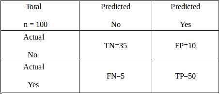
Let’s try to understand this matrix in the context of an example. Imagine you are trying to build a model to predict that a reader will be interested in reading this article or not and let’s say you are trying to classify a total of 100 potential readers. Out of those 100 readers, the classifier predicted “Yes” 60 times, and “No” 40 times. While in reality, 55 readers eventually ended up reading this article and hence were marked “Yes” and 45 readers did not read and hence were marked as “No”.
From the given information, the following terms could be defined :
True Positives (TP): These are cases in which you predicted Yes (the reader will read the article), and were actually labeled Yes (reader actually read the article).
True Negatives (TN): You predicted No (the reader will not read the article), and they were actually labeled No (reader did not read the article).
False Positives (FP): You predicted Yes, but they were labeled as No (also known as a Type I error)
False Negatives (FN): You predicted No, but they were actually labeled Yes (also known as a Type II error)
- Accuracy: Perhaps the most commonly used metric is accuracy. Mathematically defined as (TP+TN)/Total. It tells you how often the classifier is correct in making the predictions. In this example accuracy = 50+35/100 = 0.85.Generally, it is not advised to judge your model on accuracy in case of imbalanced class datasets as you can get high accuracy just by predicting all the observations as the dominant class.
- Precision: It answers the question: When the classifier predicts yes, how often is it correct? Mathematically calculated as TP/predicted Yes. In this example, precision = 50/(50+10) = 0.83.
- Recall: It answers the question: When it’s actually Yes, how often does the classifier predict yes? Mathematically calculated as TP/actual Yes. In this example, recall = 50/(50+5) = 0.90.
- False Positive Rate (FPR) : It answers the question: When it’s actually no, how often does the classifier predict Yes? Mathematically calculated as FP/actual No. In this example, precision = 10/(35+10) = 0.22.
- F1 Score: This is a harmonic mean of the Recall and Precision. Mathematically calculated as (2 x precision x recall)/(precision+recall). There is also a general form of F1 score called F-beta score wherein you can provide weights to precision and recall based on your requirement. In this example, F1 score = 2×0.83×0.9/(0.83+0.9) = 0.86
Of course, there are various other metrics you can choose to judge the performance of your model like Misclassification rate, Specificity, etc. but they are more or less related to the metrics defined above and can be looked at in conjunction with them. Try to keep things simple, don’t get confused with these terms, and most importantly try to understand the meaning of the metrics rather than cramming them up.
-
Receiver Operator Characteristic (ROC) Curve
Whenever you apply a classifier to assign a label against an observation, the classifier generates a probability against the observation and not the label. The probability is the indicator of how confidently you can assign a label against the observation and then after comparing it with a preset threshold value you assign the label to it. If you relax your threshold to a lower value, your test observations will have more number of readers labeled as Yes. The controlling threshold depends on the use case. For example, in the advertisement industry, your goal is to capture the maximum number of people who will click on the ad. Therefore, you can relax your threshold while predicting so that you can target more people.
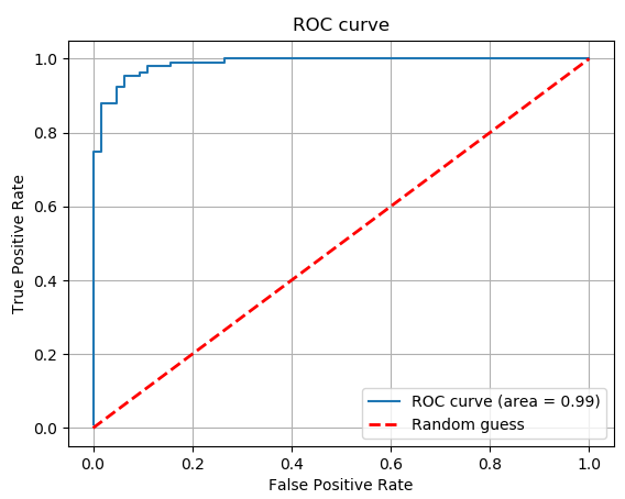
ROC or Receiver Operator Characteristic curve is a plot of the Recall (True Positive Rate) (on the y-axis) versus the False Positive Rate (on the x-axis) for every possible classification threshold.
The reason why you should check the ROC curve to evaluate a classifier instead of a simpler metric such as accuracy is that a ROC curve visualizes all possible classification thresholds, whereas accuracy only represents performance for a single threshold. Typical ROC curve looks like the image shown below:

You would want to try to build a model that produces a ROC curve that is close to the upper left corner or in other words which have maximum Area Under the Curve (AUC). Also, if your AUC is less than 0.5 i.e. the ROC curve falls below the red line then your model is even worse than a model which is based on random guesses.
One important thing to know before understanding ROC curves is the concept of the threshold.
All the metrics discussed above can be extended to a multi-class classification problem as well by using a one-versus-all approach wherein you club all the other classes except one as a separate class and repeat this process.
-
Precision-Recall (PR) Curve
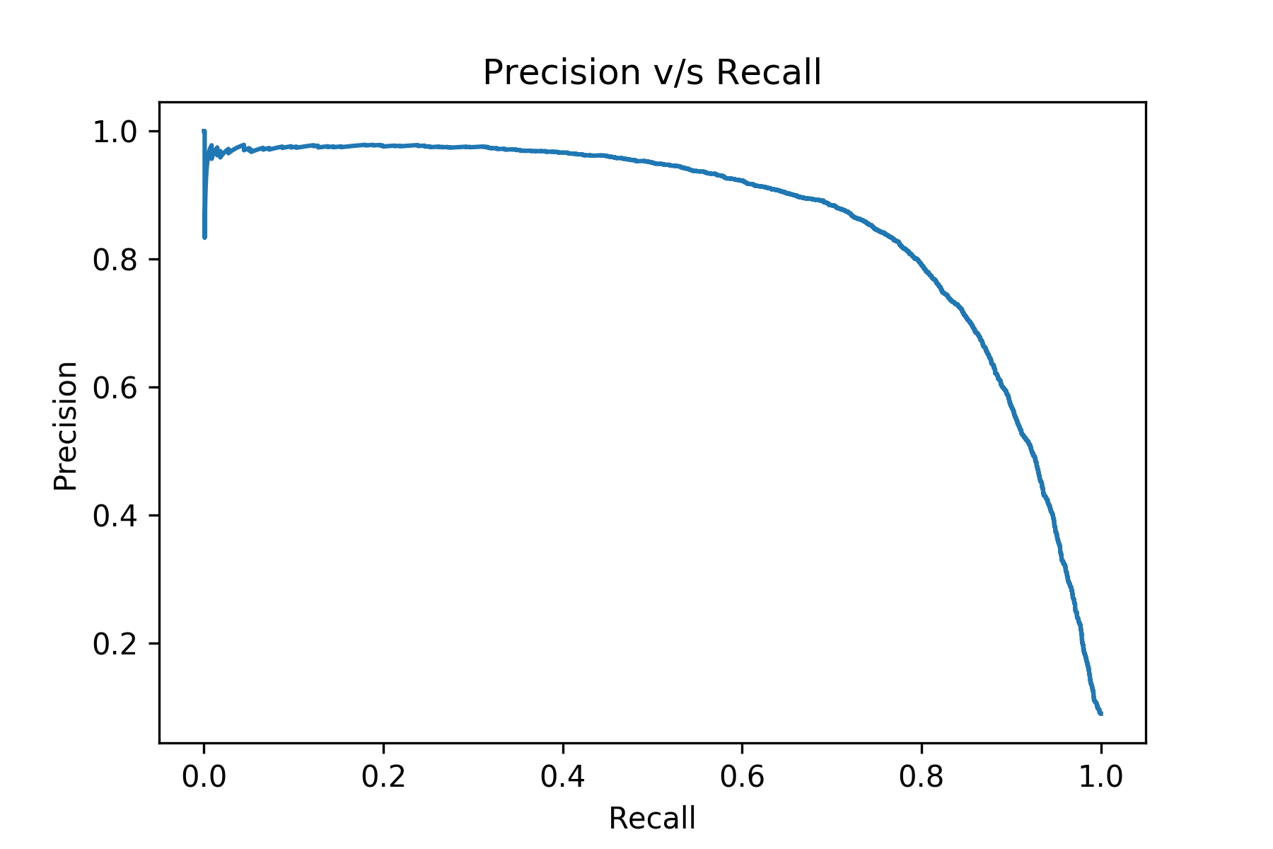
Another curve that is used to evaluate the classifier’s performance as an alternative to a ROC curve is a precision-recall curve (PRC), particularly in the case of imbalanced class distribution problems. It is a curve between precision and recall and typically looks like :

A good classifier will produce a PR-curve that is close to the upper right corner.
-
Logarithmic Loss
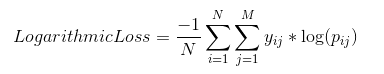
Logarithmic Loss or Log Loss, tells you how confident the model is in assigning a class to an observation. If you use Log Loss as your performance metric you must assign a probability to each class for all the samples. For any given problem, a lower log-loss value means better predictions. One important point to note about Log-loss is that it heavily penalizes classifiers that are confident about an incorrect classification. For example, if you predicted a probability of say 0.8 for a reader who read this article (1) then your log-loss will be small as your model is predicting high probability for positive class (1). But if you predict a lower probability, say 0.1, for a reader who reads this article (1) then log-loss will be greater.
Suppose, there are N samples belonging to M classes, then the Log Loss is calculated as below:

where,
𝑦𝑖𝑗 indicates whether sample i belongs to class j or not
𝑝𝑖𝑗 indicates the probability of sample i belonging to class j
The range of Log Loss is [0, ∞).
Regression Performance Evaluation Metrics
Another common type of machine learning problems in regression problems. Here, instead of predicting a discrete label/class for an observation, you predict a continuous value. For example, predicting the selling price of a house is a regression problem. A regression problem can be a linear or non-linear regression problem.
The following metrics are most commonly used to evaluate a regression model:
-
Mean Absolute Error (MAE)
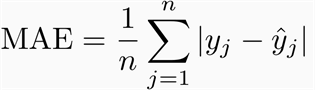
Mean Absolute Error is the average of the difference between the original value and the predicted value. It gives you the measure of how far the predictions are from the actual output and obviously, you would want to minimize it. However, it doesn’t give you an idea of the direction of the error since you are taking only the absolute values. It doesn’t penalize large errors as much as compared to RMSE. Mathematically, it is represented as:

where,
n is the number of observations
𝑦𝑗 is the actual value for sample j
𝑦̂ 𝑗 is the predicted value for sample j
For example, let’s pick a regression problem where you are trying to predict the number of readers of this article, and let’s say your test set has two observations only, meaning n= 2. If actual number of readers, 𝑦𝑗 = [10,5] and your model predicts, 𝑦̂ 𝑗 = [8,6] readers then MAE = (½) * (|10-8| + |5-6|) = 1.5.
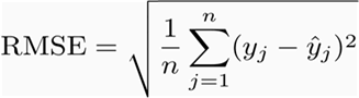
- Root Mean Squared Error (RMSE)

For the example discussed in MAE section, RMSE = ((½) * ( (10-8)^2 + (5-6)^2))^(½) = 1.581.Perhaps the most popular evaluation metric used to evaluate regression problems is RMSE. Mean Squared Error (MSE) is similar to MAE, the only difference being that MSE takes the average of the square of the difference between the original values and the predicted values which eases the process of gradient calculation, penalizes the error terms more, and is unbiased towards the direction of error (since you are squaring). However, this makes it more sensitive to outliers. Mathematically, it is represented as:
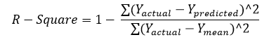
- R Squared / Coefficient of Determination
Often used in the case of Linear Regression problems, R squared determines how much of the total variation in Y (dependent variable) is explained by the variation in X (independent variable).
Mathematically, it can be written as:

For the example described above, Yactual = 𝑦𝑗 = [10,5] ; Ypredicted = 𝑦̂ 𝑗 = [8,6] and Ymean = 10+5/2 = 7.5. You can plug these values inside the formula and you will notice your R squared = 0.6
A higher R-squared is preferable while doing linear regression. The range of R-square is (- ∞,1] (don’t get confused by the name, r-squared, it can be negative as well!). While a high r-square value gives you a sense of the goodness of fit of the model, it shouldn’t be used as the only metric to pick the best model. If you care about the absolute predictions then probably it’s better to check RMSE/MAE as well.
-
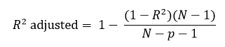
Adjusted R Square

The drawback of R-Square is that if you add new predictors (X) to your model, the R-Square value only increases or remains constant but it never decreases because of which you cannot judge that by increasing the complexity of your model, are you making it more accurate? That is where Adjusted R-squared comes in, it increases only if the new predictor improves model accuracy. (Python users might have to code this explicitly as of now!)
Clustering Performance Evaluation Metrics
Clustering is the most common form of unsupervised learning. You don’t have any labels in clustering, just a set of features for observation and your goal is to create clusters that have similar observations clubbed together and dissimilar observations kept as far as possible. Evaluating the performance of a clustering algorithm is not as trivial as counting the number of errors or the precision and recall like in the case of supervised learning algorithms.
Here clusters are evaluated based on some similarity or dissimilarity measure such as the distance between cluster points. If the clustering algorithm separates dissimilar observations apart and similar observations together, then it has performed well. The two most popular metrics evaluation metrics for clustering algorithms are the Silhouette coefficient and Dunn’s Index which you will explore next.
-
Silhouette Coefficient

The Silhouette Coefficient is defined for each sample and is composed of two scores:
a: The mean distance between a sample and all other points in the same cluster.
b: The mean distance between a sample and all other points in the next nearest cluster.The Silhouette Coefficient for a set of samples is given as the mean of the Silhouette Coefficient for each sample. The score is bounded between -1 for incorrect clustering and +1 for highly dense clustering. Scores around zero indicate overlapping clusters. The score is higher when clusters are dense and well separated, which relates to a standard concept of a cluster.
-
Dunn’s Index
Dunn’s Index (DI) is another metric for evaluating a clustering algorithm. Dunn’s Index is equal to the minimum inter-cluster distance divided by the maximum cluster size. Note that large inter-cluster distances (better separation) and smaller cluster sizes (more compact clusters) lead to a higher DI value. A higher DI implies better clustering. It assumes that better clustering means that clusters are compact and well-separated from other clusters.
End Notes
So this brings us to the end of this article. This article was written with the sole purpose to cover the most important and most commonly used machine learning model evaluation metrics and bring some clarity towards the meaning of these evaluation metrics. I hope this might have helped you in some way and motivated you to pick up the right metric for your use-case in order to evaluate how good a machine learning model you have built.