This article was published as a part of the Data Science Blogathon
Hi, all Analytics Vidhya readers. Hope you all are doing well in this hard time of the Covid era.
In this article, we are going to predict the wind speed of the current date and time for any given latitude and longitude coordinates. We’ll be using a K-neighbors classifier to build our predicting model. The dataset we are using is available on GitHub here.
Starting with our task
The first step which I always suggest is to check the python version which you are using. I am using an anaconda package and a jupyter notebook. So whichever editor you are using, type in the following
from platform import python_version
print(python_version())
The output will be. I am using Python version 3.8.8 as shown here.
3.8.8
Importing important libraries-
The first step is to import libraries. We are using pandas, numpy, scikit-learn and datetime modules to analyse our dataset.
import pandas as pd
import numpy as np
from sklearn.model_selection import train_test_split
from sklearn import metrics
from sklearn.neighbours import KNeighborsClassifier
from datetime import datetime
Reading the dataset-
The second step is to read the data file which we are going to analyse. The file is in .csv format.
data = pd.read_csv('sat.csv')
data.info()
The output of the above code is:
RangeIndex: 72890 entries, 0 to 72889
Data columns (total 4 columns):
 #   Column      Non-Null Count  Dtype
---  ------      --------------  -----
 0   X           72890 non-null  float64
 1   Y           72890 non-null  float64
 2   time        72890 non-null  float64
 3   wind_speed  72501 non-null  float64
dtypes: float64(4)
memory usage: 2.2 MB
If you see the output following things can be analysed:
- There are 72890 entries in the dataset.
- There are 4 columns: X, Y, time and wind_speed.
- The data type is float.
- Some values are missing in the wind_speed column. We’ll analyse this in a while.
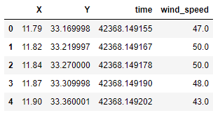
Let’s print the first 5 values of our dataset.
data.head()
The output is:

OK. So, X and Y correspond to latitudes and longitudes coordinates respectively. If we closely see the time column the entries are written in epoch timestamp. To predict the wind speed of the current duration, we need to determine what time this epoch timestamp is showing. For this, the datetime module is quite handy.
Let’s take the first value from the time column and see what time and date it is pointing.
timestamp = 42368.149155
#convert timestamp to datetime object
dt_object = datetime.fromtimestamp(timestamp)
print("dt_object:", dt_object)
The output of the above code is:
dt_object: 1970-01-01 17:16:08.149155
If we see the output, the timestamp is pointing at the year 1970, January 01, and the timing is 17:16:08.149155. Now we can also convert the time column data into date-time value like this.
for i in data['time']:
    dt_object = datetime.fromtimestamp(i)
    print(dt_object)
We can create a new column and it in the existing dataset also. This will help to analyse timestamp and time relation properly.
data['Time_Analysis'] = pd.to_datetime(data['time'], unit='s')
Note that, I am using unit = ‘s’. This will help to convert the time into standard GMT otherwise the output will be in IST. If you want to use IST, don’t write unit = ‘s’. If we again see the first 5 values now using
data.head()
Executing this, we have,

We can see that the data is of January only and the difference is in seconds only between two data points.
Data Cleaning
Now moving on, we aim to determine the wind_speed. And previously we saw that the wind_speed column has some missing data in it. So, let’s analyse it. If we check for the presence of null values and sum it, we can see that there are 389 rows with no entries in them.
data.wind_speed.isnull().sum()
The output is:
389
What I’ll do, I’ll drop these 389 values. One can also use interpolation techniques and fill these empty cells with methods like forward-fill, backwards-fill, etc. But for the time being, let’s drop these rows.
data = data.dropna(how = 'any', axis = 0)
OK. Now it’s time to train our data. Starting with the first step of feature selection.
Feature and Target selection-
Our target is to find the wind speed so that will be the target or our dependent variable. To determine the wind speed we need X, Y and time, so they will be our features.
If we check the shape of the data, we see that there are 72501 rows and 5 columns.
data. shape
And the shape of the data is
(72501, 5)
Remember that, we have drop 389 empty cells. That’s why 72501 rows are present. Let’s assign the feature and target samples now.
feature_col = ['X', 'Y', 'time']
target = ['wind_speed']
Also, we can see the shapes of our feature dataset and target dataset. Let X be the variable assigned for the feature dataset and y be the target dataset.
X = data[feature_col]
print(X.shape)
The output shapes are,
(72501, 3) # feature dataset shape
(72501, 1) # target dataset shape
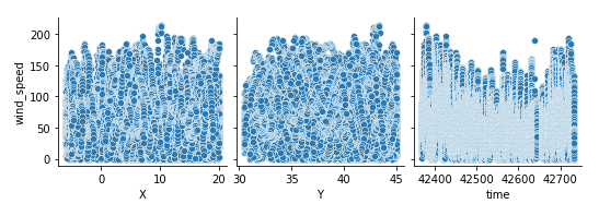
We can also visualize our dataset. For this, I am using the seaborn data visualization library.
import seaborn as sns
%matplotlib inline
sns.pairplot(data, x_vars = ['X', 'Y', 'time'], y_vars = 'wind_speed')
If we observe, the data is approximately uniform.

You can see some variation in wind_speed vs. time graph, but don’t forget that this graph has values changing over fractions of seconds. Over a long duration of time, we can consider it uniform.
Splitting the data into training and testing dataset
Using the train_test_split function we can now split our dataset into training and testing datasets. I’ll be using the default values only. but one can split the dataset according to their need.
X_train, X_test, y_train, y_test = train_test_split(X, y, random_state = 1)
print(X_train.shape)
print(X_test.shape)
print(y_train.shape)
print(y_test.shape)
Just, in brief, let me explain what these terms mean:
- X_train- it has all the feature variables, a fraction of which are used to train the model.
- X_test- it also has all the feature variables which were left from training.
- y_train- it is the target data that will be predicted by the ML model. At the time of training itself, the target variable is set.
- y_test- it is used to test the accuracy between actual and predicted values.
And printing the shapes will give the dimensions of the training and testing dataset.
(54375, 3) # X_train shape
(18126, 3) # X_test shape
(54375, 1) # y_train shape
(18126, 1) # y_test shape
We can observe that by default, 75% of data is used for training and 25% of data is used for testing. Now it’s time to implement our machine learning model. We are using K-neighbors classifier for this. Let’s get a very brief introduction to K-Neighbors classifier.
According to Wikipedia, “In statistics, the k-nearest neighbour’s algorithm (k-NN) is a non-parametric classification method first developed by Evelyn Fix and Joseph Hodges in 1951 and later expanded by Thomas Cover. It is used for classification and regression. In both cases, the input consists of the k closest training examples in the data set. The output depends on whether k-NN is used for classification or regression. In k-NN regression, the output is the property value for the object. This value is the average of the values of k nearest neighbours.“
In our case, we are dealing with a regression problem and the number of neighbours we are choosing is 1.
knn = KNeighborsClassifier(n_neighbors = 1)
knn.fit(X,y)
On running we are not getting any errors. That’s good, but we are getting some warning.

We can remove the warning. This can happen sometimes if you have float data. The solution is also provided in the warning itself.
knn = KNeighborsClassifier(n_neighbors = 1)
knn.fit(X,y.values.ravel())
OK, now the warning is also removed. Let’s check if our model is working correctly or not. For that first, I am using the first row data.

So, we’ll use these values of X, Y and time and see if we get this wind_speed or not. We can directly use any values straight away, but this will help us to see if our model is giving correct predictions or not.
check_coord = [[11.79, 33.169998, 42368.149155]]
print(knn.predict(check_coord))
The output we are getting is:
[47.]
So our model is predicting correctly. We can measure the accuracy also.
y_pred = knn.predict(X)
print(metrics.accuracy_score(y,y_pred))
And the output is:
1.0
An accuracy of 1.0 means 100%. So, our model is predicting with 100% accuracy. What if we have neighbours = 5?
knn = KNeighborsClassifier(n_neighbors = 5)
knn.fit(X,y.values.ravel())
print(knn.predict(check_coord))
The output is:
[50.0]
Again checking the accuracy,
y_pred = knn.predict(X)
print(metrics.accuracy_score(y,y_pred))
And the accuracy is:
0.3469055599233114
The accuracy, in this case, is very poor, around 34%. So, we’ll use neighbours value equal to 1.
So now we can check it on any coordinates. Let’s take some random coordinates which are not present in our dataset. Let X = 23.1 and Y = 79.9. First, check whether these coordinates are present in our dataset or not.
data.loc[(data['X'] == 23.1) & (data['Y'] == 79.9)]
As we can see, there are no such coordinates and hence nothing is displayed.

Now we have some random X Y coordinates and to determine wind_speed for these coordinates, we need time. For this model, we are interested in the current timestamp. using any online epoch converter, we can check what is the timestamp value for the current time and date. If we check the current timestamp value is 1627112345. Let’s verify it with the datetime module.
from datetime import datetime
timestamp = 1627112345
#convert timestamp to datetime object
curr_time = datetime.fromtimestamp(timestamp)
print("Current Time:", curr_time)
OK. The output is:
Current Time: 2021-07-24 13:09:05
Now we have X, Y and time features and we can straight away put these into our model to determine the wind speed. Remember to take neighbours value equal to 1.
new_coord = [[23.1, 79.9, 1627112345]]
print(knn.predict(new_coord))
[26.] # output
Again, let’s check the accuracy
y_pred = knn.predict(X)
print(metrics.accuracy_score(y,y_pred))
The accuracy obtained is:
1.0
So, our model is predicting the wind speed with 100% accuracy. This is how we can use latitude, longitude and time to predict wind_speed.
Conclusion:
In this article, we have learned how to read data using. CSV files, how to clean data eliminating unwanted data, how to split data into training and testing datasets and then training the model to predict the output. We also learn to determine the accuracy of the predicted output.
We can use other interpolation techniques to check for other possibilities. I used Naive Bayes Classifier and Logistic Regression methods also. You can try with other learning models. I hope this article explains all the steps required to learn prediction using the K-neighbors classifier. If you liked this article then please share it with your friends. Learning is sharing more knowledge.
Thanks for reading this post. Have a great time ahead !!!
About the Author-
Hi all Geeks. I am Abhishek Singh, Assistant Professor, Electronics and Communication Engineering Department, Gyan Ganga Institute of Technology and Sciences, Jabalpur, MP. I am Data Scientist, YouTuber, Content Writer, Blogger, Python Editor and Author. I love to teach Electronics, Python and VLSI. Please feel free to contact me through-
Thank You!!!


