Introduction
In today’s world, machine learning and artificial intelligence are widely used in almost every sector to improve performance and results. But are they still useful without the data? The answer is No. The machine learning algorithms heavily rely on data that we feed to them. The quality of data we feed to the algorithms highly determines the results and performance of the machine learning models. The problem is the available data is rarely perfect. Hence, we have to modify the dataset to take the most benefit out of it.

Learning Objectives
In this article, we will talk about one such interesting dataset using machine learning and see how we can modify it to make it close to perfect. We will learn about
1. Some interesting libraries in python to modify the dataset, create the model and evaluate it.
2. How to perform exploratory data analysis and feature engineering?
3. How to deal with outliers?
4. What is Sampling, and how is it performed?
This article was published as a part of the Data Science Blogathon.
Table of Contents
- What is the Project About?
- Problem Statement
- Before You Go Further, Know Some Prerequisites!
- Knowing More About the Dataset
- EDA and Target Data Analysis
- Finding Outliers in Dataset
- Transforming Features With Feature Engineering
- It’s Cold! Where’s the Heatmap?
- Modeling
- Is the Data Good Enough?
- Removing The Imbalance from the Dataset
- Understanding Sampling of Data
12.1 Undersampling
12.2 Oversampling - Conclusion
What is the Project About?
Insurance policies are a great way for anyone who is looking to protect their family and assets from financial risks and losses. These plans help you pay for any medical care and emergencies. In the case of vehicle insurance policies, it helps to pay for any vehicle damage or damage caused by the vehicle. The law mandates that every motor vehicle owner have a motor insurance policy. In exchange for the guarantee of compensation against these losses, the insurance companies ask its customer for a small premium amount. Although the risks are high, the probability of these damages is very low, say 2 in 100. This way, everyone shares the risk of everyone else.

Source: dreamstime
The insurance companies that provide these medical and vehicle insurances highly rely on machine learning to improve customer services, operational efficiency, and fraud detection. The company uses the user’s experience to predict whether there will be mishappening caused by that customer or to the customer. The company may gather details like age, gender, health status, history, etc., before issuing any insurance policy.
Problem Statement
In this article, we’ll be using vehicle insurance data to predict whether a customer will be interested in buying the vehicle’s insurance policy or not. Ideally, the dataset we use in machine learning should have a balanced ratio of target variables for the model to give unbiased results. But as we discussed earlier, the probability of happening of any accident in a sample population is significantly rare. Similarly, the chances for a person interested in buying an insurance policy from a sample of people are quite low. Therefore, the dataset we are using in this article is highly imbalanced, and we will see how using the dataset as it is will result in poor and biased results. Therefore, we will have to apply techniques to balance the data first before moving on to the modeling part.
Before You Go Further, Know Some Prerequisites!

For this project, you should have a basic understanding of python and libraries like Pandas, Numpy, and Sklearn. You should know basic terms used in machine learning, such as train and test data, model fitting, classification, regression, confusion metrics, and basic machine learning algorithms like logistic regression, K nearest neighbors, etc. Moreover, a rough idea of exploratory data analysis and plotting libraries like Matplotlib and seaborn would be beneficial.
Knowing More About the Dataset
The dataset we will use in this article is imbalanced insurance data. The dataset can be downloaded through this link. The aim of using this dataset is to predict whether a customer will be interested in buying vehicle insurance or not. To predict this customer behavior, there are several features in the dataset. The dataset includes demographic information of customers like their age, gender, area code, vehicle age, vehicle damage, etc. It also contains information such as whether the customer has previously bought insurance or not, what premium the customer is paying, and the policy sales channel. The target variable in this dataset is the Response variable which denotes whether the customer has bought the vehicle insurance or not.
The dataset contains 3,82,154 rows and 12 columns, including the Response variable. To learn more about the dataset, we’ll use some basic functions in pandas.
Python Code:
In the above snippet, we have used pandas.DataFrame.head() function to get the top 5 observations in the dataset. This will help us get a little idea about what kind of values we will be dealing with. Similar to the head function, you can use pandas.DataFrame.tail() function to get the end 5 values in the dataset. You can give a number in the function as an argument if you want to get more or less several rows.

The pandas.DataFrame.shape allows us to get the structure of the dataset. We now know that the dataset contains 12 columns and 3,82,154 records.

The Pandas.dataFrame.describe() function gives a lot of insights about the dataset. This functionality returns the descriptive statistics of the dataset, giving us an idea about the distribution’s frequency, central tendency, and dispersion. This function is very helpful, although a little care should be taken because some of the values might not make sense. For example, in the dataset, region code is a nominal variable (the data that can be categorized but cannot be ranked), and its mean value doesn’t make sense. But the describe function assumes it as an integer value and returns the average region code and standard deviation of region code, which sounds ridiculous itself.
EDA and Target Data Analysis
We have now understood the problem statement and know something about the dataset. We have a good start, but there’s much more to learn about the dataset. Let’s first check if the dataset contains any null values.
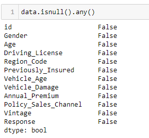
From the above snippet, it’s clear that the dataset doesn’t contain any null values. However, if your dataset does contain null values, then you should go through this link.
Next, we will analyze the target variable, which is the Response variable. We will see how the Response variable is distributed across the dataset.
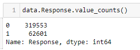
From the above snippet, we can see the value counts of the Response variable. We see that the Response variable is highly imbalanced with 0 which is No response being the majority class. The 0 class represents that the customer is not interested in taking the insurance, whereas 1 denotes the customer is interested. Let’s see the ratio of this distribution using a pie chart. This is where we use the plotting library matplotlib.
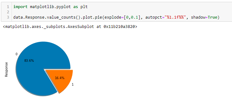
To learn more about the parameters of the matplotlib pie chart, refer to this link. From the above pie chart, we can see the ratio in which the Response class is distributed is almost 84:16. In reality, the dataset could be more imbalanced. So, to make it more interesting we will drop some values from the positive class.
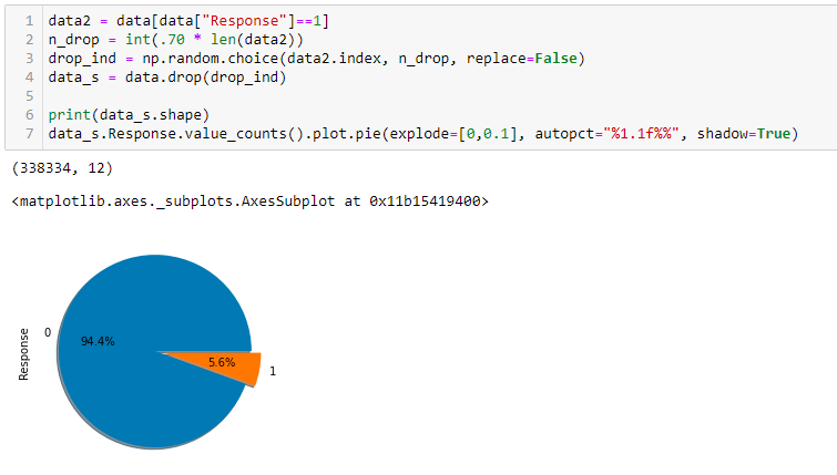
We randomly selected and dropped 70% of values from the positive class, and now as you can see, the imbalance ratio is 95:5.
Finding Outliers in Dataset
In this step, we will look for outliers in the dataset. An outlier is an observation that seems abnormal from the other values in a population. The reason for outliers could be data entry errors, sampling problems, and unusual conditions. Dealing with outliers is important as it decreases the statistical power and increases variability in the dataset.
Usually, it is best not to remove the outliers to make a better fitting model, as it may lead to the loss of crucial legitimate information. However, in this article, our main aim is to learn about dealing with imbalanced data, and the data points are plenty. Hence, we can think about dropping the outliers. You can refer to this link to learn how to deal with outliers.
We will use the interquartile range method to find outliers in our dataset. The interquartile range contains the values where the second and third-quarter values of the dataset lie. Any values that lie outside (q1-1.5*IQR) and (q3+1.5*IQR) is considered an outlier.
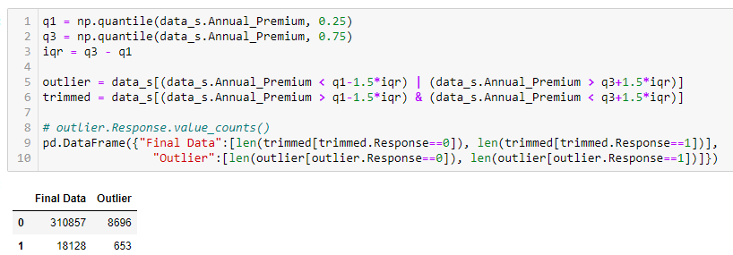
As you can see in the above snippet, there are around 9000 outliers in the dataset. Compared to the size of the original dataset, the size of outliers is quite small. Hence, we can remove those outliers from the dataset. We found almost 8500 outliers in the negative class, whereas around 600 are in a positive class. So, after removing these outliers, the final size of the dataset has 3,10,857 values for the positive Response class and 18,147 values for the negative Response class.
Transforming Features With Feature Engineering
In this step, we will deal with the categorical data in the dataset. The Gender and the vehicle damage feature of the dataset have binary data; that is, there are only two possible values. So, in the case of Gender, we have assigned males 1 and females 0. Similarly, we assigned yes as 1 and no as 0 in case of vehicle damage. Then, we changed the data type of the feature from a string to an integer.
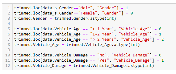
If we look closer into the dataset, we will find that the Region code contains float values. As the Region code is nominal (meaning we can’t rank the region code, and we can’t compare or take an average of the region code ), the float value doesn’t make sense. Hence, we change its data type to int.
The id variable in the dataset contains the unique key of the user. Hence it won’t do much help in the prediction of the response. So, we will drop the id column from the dataset.

It’s Cold! Where’s the Heatmap?
In this part, we will see how the features are correlated to each other and how they impact the response variable. To do this, we will create a heatmap using the matplotlib and the seaborn library in python. A heatmap is a 2-dimensional graphical representation of data where individual values are contained in a matrix and are represented in the form of colors. The lighter shades represent the values positively correlated with each other, whereas the darker shade represents the values negatively correlated with each other. A heatmap is a great way to find the most significant elements in a dataset and is used to find interesting trends across the data.
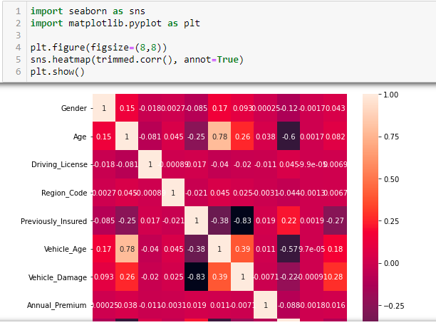
In the above image, you can observe every value is perfectly correlated with itself, hence the value 1. You can observe that the Previously insured feature and Vehicle Damage show a comparatively high correlation with the response variable. The other values show little correlation, but we can still use them for the modeling part.
Modeling
We will split our dataset into train and test data in this part. We will use the training data for our machine learning and model, then test how well it performs on the test data. We will use 70 percent of the data for training and save 30 percent for testing purposes. We will use the sklearn library’s train test split function to perform this.

Is the Data Good Enough?
Before dealing with the imbalanced data, we will first create a function to evaluate the dataset. This way, we can easily evaluate the techniques we will use to balance the data.
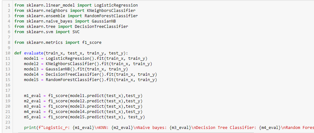
We will create an evaluation function and use five machine-learning algorithms to make predictions in the test data. These algorithms are Logistic regression, K Nearest Neighbors Classifier, Decision Tree Classifier, Naïve Bayes Classifier, and Random Forest Classifier. To check if the predictions are correct, we will use the f1 score metrics.
To define how well a classification algorithm performs, confusion metrics are used. We are not going into detail about what a confusion matrix is. In brief, the confusion matrix compares the values that the model and the actual values predict. It can be used to find accuracy, precision, recall, and the f1 score. You can refer to this link to learn about the confusion matrix.
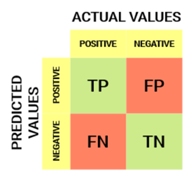
Generally, we use accuracy metrics to know how well the model performs. But, if you go through the above link, you will find that using the f1 score is a better metric than the accuracy in the imbalanced dataset. In brief, the accuracy score doesn’t help to know whether the model works great for both classes. In contrast, the f1 score helps to determine the model’s performance for each Response class.
Now we will use the sklearn library to import the machine learning algorithms and the f1 score that we will use to measure the efficiency.
Removing the Imbalance from the Dataset
Now comes the part where we will deal with the imbalance in the dataset. But the question arises, what happens if we use the imbalance data as it is for training?
Using the data as it is may give a good accuracy score, but as discussed earlier, accuracy isn’t the right metric when dealing with imbalanced data.

The above snippet shows that the f1 score is almost 0 for logistic regression, KNN, and random forest classifiers. Hence, we can conclude that we can’t use the data as it is, and dealing with the imbalanced data is a must.
There are two effective ways of dealing with imbalanced data Sampling and Upweighting. In this article, we will talk about sampling and various techniques that fall within sampling.
Understanding Sampling of Data
Data sampling is a statistical technique used to manipulate and analyze a subset of data points to identify patterns in a larger set. It can be achieved by reducing samples from the majority class or increasing samples in the minority class. One important thing to remember in sampling is that it is applied only to the training data to influence the machine learning model. The test data remains untouched while sampling.
Undersampling
Undersampling is a technique that is used to balance an uneven dataset. This technique is used when the dataset contains plenty of data points. Here, the size of the majority class is decreased by removing some samples from the majority class without making any changes in the minority class to make it balanced. This is a very useful technique. However, it leads to loss of information and is thus avoided when the dataset already has very few data points.
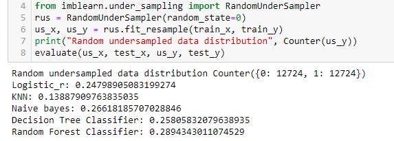
Random Under Sampling
Under-sampling is an under-sampling technique in which samples are selected randomly from the majority class and deleted from the training data. It is also referred to as naïve sampling as it takes no assumptions about the data. This technique is fast and simple to implement and hence opted often for complex and large datasets. It can be used for binary or multi-class classification, which may have one or more minority or majority classes.
As discussed earlier, random under-sampling may lead to the loss of useful information in the dataset. One way to deal with this is by using the sampling strategy. Using the sampling strategy, we can provide the desired ratio of minority to majority classes. Hence, we can decide how much we can bear the data loss.
Nearest Neighbor Resampling
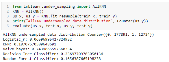
This resampling uses the nearest neighbors algorithm to remove the samples which do not agree with their neighborhood. This includes several variants of algorithms like edited nearest neighbors, repeated edited nearest neighbors, and All KNN. These algorithms can be performed on the entire dataset or, specifically, on the majority class.
Oversampling
Oversampling is the technique opposite to undersampling. In this technique, we reproduce the samples from the minority class and increase the minority class dataset. This new minority data can be added by random generation (Random Oversampling) or mathematical calculations (SMOTE Sampling). Oversampling is extremely useful; however, it makes the dataset prone to overfitting.
Random Over Sampling
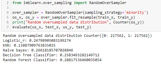
Random oversampling is similar to random undersampling. Instead of removing the samples from the majority class, it randomly selects them from the minority class and creates duplicates. Hence, increasing the size of the minority class. It’s fast and easy to implement. However, it can lead to overfitting. Hence, we can use a sampling strategy to under-sample and oversample.
SMOTE (Synthetic Minority Oversampling Technique)
It is one of the most common over-sampling techniques. It replicates the minority class samples by linear interpolation of the minority class. This technique generates synthetic training records by randomly selecting one or more k nearest neighbors from the minority class. This approach is effective as it adds new synthetic samples from the minority class that are plausible and relatively close to the existing samples. Although, there is one downside of this algorithm it doesn’t consider majority class samples into consideration. Hence, there is the possibility of having ambiguous records if there is a substantial overlap between the classes.
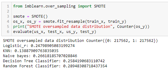
Undersampling followed by Oversampling
Now we know the pros and cons of both undersampling and oversampling, we can use them together to take the most out of it. We can either manually apply to undersample followed by oversampling or use the imblearn library for that.
First, we will combine SMOTE oversampling along with random undersampling. Here, we will use a sampling strategy as we don’t want to resample the whole data simultaneously. This parameter can be tuned to change the data distribution and improve the final scores.

Next, we will use SMOTE oversampling along with the nearest neighbor undersampling. This combination has already been implemented in the imblearn library and is proven to be an efficient sampling method. The Edited nearest neighbor uses the 3 nearest neighbors to locate those misclassified samples in the dataset.
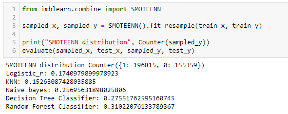
Now we have seen several ways to balance our data. It depends on you which technique you use. But you should be unbiased towards a technique and analyze the dataset first, to understand the requirements and to get the best out of all. You can tune the sampling strategy parameter to improve the results to your requirement. If you want to learn more sampling techniques, you can refer to the original documentation of the imblearn library.
Conclusion
Source: freepowerpointtemplates.com
In this article, we learned about an interesting dataset of vehicle insurance using machine learning. We saw how one class is majorly distributed across the dataset while the other rarely exists in the data. We performed exploratory data analysis on the data and applied feature engineering. We learned why this imbalanced data couldn’t be treated like a balanced dataset. Even the metrics used to evaluate the imbalanced data differ from the ones used in the balanced data. We looked at how to deal with the imbalance in the data.
Key Takeaways
1. You know about several algorithms that can be used to balance this data, which can only be used for modeling.
2. You saw how the model’s performance changes when the dataset is used as it is versus when it is modified using sampling techniques.
3. You learned about each algorithm’s pros and cons; at last, we tested if combining those sampling algorithms gives better results.
You can find this article’s code in this git hub repo. After reading this article, I hope you know how to deal with an imbalanced dataset.
You can see more of my articles here.
You can connect with me on Linkedin.
The media shown in this article is not owned by Analytics Vidhya and is used at the Author’s discretion.


