This article was published as a part of the Data Science Blogathon
Naive Bayes Classifier Overview
Assume you wish to categorize user reviews as good or bad. Sentiment Analysis is a popular job to be performed by data scientists. This is a simple guide using Naive Bayes Classifier and Scikit-learn to create a Google Play store reviews classifier (Sentiment Analysis) in Python.
Naive Bayes is the simplest and fastest classification algorithm for a large chunk of data. In various applications such as spam filtering, text classification, sentiment analysis, and recommendation systems, Naive Bayes classifier is used successfully. It uses the Bayes probability theorem for unknown class prediction.
The Naive Bayes classification technique is a simple and powerful classification task in machine learning. The use of Bayes’ theorem with a strong independence assumption between the features is the basis for naive Bayes classification. When used for textual data analysis, such as Natural Language Processing, the Naive Bayes classification yields good results.
Simple Bayes or independent Bayes models are other names for nave Bayes models. All of these terms refer to the classifier’s decision rule using Bayes’ theorem. In practice, the Bayes theorem is applied by the Naive Bayes classifier. The power of Bayes’ theorem is brought to machine learning with this classifier.
Naive Bayes algorithm intuition
The Bayes theorem is used by the Naive Bayes Classifier to forecast membership probabilities for each class, such as the likelihood that a given record or data point belongs to that class. The most likely class is defined as the one having the highest probability. The Maximum A Posteriori is another name for this (MAP).
For a hypothesis with two occurrences A and B, the MAP is
MAP (A)
= max (P (A | B))
= max (P (B | A) * P (A))/P (B)
= max (P (B | A) * P (A)
All of the features in the Naive Bayes Classifier are assumed to be unrelated. A feature’s presence or absence has no bearing on the presence or absence of other features.
We test a hypothesis given different evidence on features in real-world datasets. As a result, the computations become fairly difficult. To make things easier, the feature independence technique is utilized to decouple various pieces of evidence and consider them as separate entities.
Types of Naive Bayes algorithm
There are 3 types of Naïve Bayes algorithm. The 3 types are listed below:-
- Gaussian Naïve Bayes
- Multinomial Naïve Bayes
- Bernoulli Naïve Bayes
Applications of Naive Bayes algorithm
Naive Bayes is one of the most straightforward and fast classification algorithms. It is very well suited for large volumes of data. It is successfully used in various applications such as :
- Spam filtering
- Text classification
- Sentiment analysis
- Recommender systems
It uses the Bayes theorem of probability for the prediction of unknown classes.
Data Overview
Requirements
In this tutorial, we need all of the following python libraries.
pandas – Python Data Analysis Library. pandas are open-source, BSD-licensed libraries for the Python programming language that provide high-performance, simple-to-use data structures, and data analysis tools.
Numpy – NumPy is a scientific computing fundamental package in Python. It contains among other things:
- a powerful N-dimensional array object
- sophisticated (broadcasting) functions
- tools for integrating C/C++ and Fortran code
- capabilities in linear algebra, Fourier transform, and random numbers
sci-kit learn – Data mining and data analysis tools that are easy to use.
python_dateutil – The date util module extends Python’s conventional DateTime module with a number of useful features.
Pytz – is a Python package that integrates the Olson database. With Python 2.4 or above and this module, you can calculate time zones accurately and cross-platform.
Read into Python
Let’s first read the required data from a CSV file using the Pandas library.
Python Code:
Pre-process Data
Note: There are many different and more sophisticated ways in which text data can be cleaned that would likely produce better results than what I did here. To be as easy as possible in this tutorial. I also generally think it’s best to get baseline predictions with the simplest solution possible before spending time doing unnecessary transformations.
Splitting Data
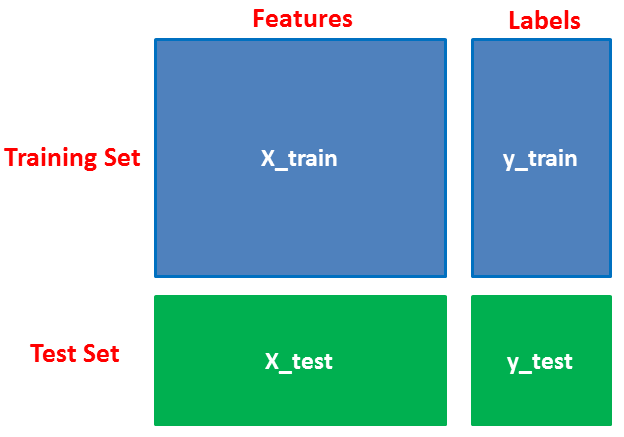
First, separate the columns into dependent and independent variables (or features and labels). Then you split those variables into train and test sets.

# Split into training and testing data
x = data['review']
y = data['polarity']
x, x_test, y, y_test = train_test_split(x,y, stratify=y, test_size=0.25, random_state=42)
Vectorize text reviews to numbers.
# Vectorize text reviews to numbers
vec = CountVectorizer(stop_words='english')
x = vec.fit_transform(x).toarray()
x_test = vec.transform(x_test).toarray()
Vectorization: To make sense of this data for our machine learning algorithm, we will need to convert each review to a numerical representation that we call vectorization.
Model Generation
After splitting and vectorize text reviews into numbers, we will generate a random forest model on the training set and perform prediction on test set features.
from sklearn.naive_bayes import MultinomialNB

model = MultinomialNB()
model.fit(x, y)
Check the correctness of the model after it has been created by comparing real and anticipated values. This model is 85 % accurate.
model.score(x_test, y_test)

Then check prediction.
model.predict(vec.transform(['Love this app simply awesome!']))
And there it is. A very simple classifier with 85% pretty decent accuracy out of the box.
EndNote
Thank you for reading!
I hope you enjoyed the article and increased your knowledge.
Please feel free to contact me on Email
Something not mentioned or want to share your thoughts? Feel free to comment below And I’ll get back to you.
About the Author
Hardikkumar M. Dhaduk
Data Analyst | Digital Data Analysis Specialist | Data Science Learner
Connect with me on Linkedin
Connect with me on Github


