This article was published as a part of the Data Science Blogathon
What is NumPy and Why NumPy is an important library to work with data?
NumPy is a Python library widely used to handle arrays with arrays. Numpy can handle oversized, multi-dimensional arrays and matrices, along with a large collection of mathematical operations to operate on these arrays. It stands for numerical python. NumPy can provide an array object that is 50 times faster than traditional Python lists.
An array occupies less memory and is extremely convenient to use as compared to python lists. Additionally, it has a mechanism for specifying the data types. NumPy can operate on individual elements in the array without using loops and list comprehensions.
Now, before diving deep into the concept of NumPy arrays, it’s important to note that Python lists can very well perform all the actions that NumPy arrays perform; it is simply the fact that NumPy arrays are faster and more convenient that lists when it comes extensive computations, which make them extremely useful, especially when you are working with a large amount of data.
Installing NumPy in your System
$ pip install numpy
Getting started with NumPy
Once Numpy is successfully installed in your system, you can import NumPy simply by
import numpy as np
where np is an alias used for NumPy so that the NumPy package can be referred to as np instead of numpy.
There are two ways to create NumPy arrays, which are mentioned below:
- By converting the existing lists or tuples to arrays using np.array
- By initializing fixed-length arrays using the Numpy functions.
#Creating a 1D numpy array
arr = np.array([1,2,3,4,5])
#Creating a 2D array
arr = np.array( [  [1,2,3],
                   [4,5,6] ] )
# Creating array of ones
np.ones(5) #1D
np.ones( (3,5) ) #2D
# Change the default dtype of an array
np.ones( (5) ,dtype = np.int) # creating array of integers
np.ones( (5) ,dtype = np.float ) # creating array of floats
# Creating array of random numbers
np.random.random( [3,4] )
#creating an array of numbers 1 to 100 with step of 5
np.arange(1,100,5)
#Creating an array of length 25 between 1 to 10
np.linspace(1,10,25)  # It equally divides 1 to 100 in 25 parts
#creating a array of particular number
np.full( ( 3,3) , 5) #It will create an array of 3x3 of 5's
# To create an array of repeating sequence
np.tile( [1,2,3] , 3 ) # The op will look like [ 1,2,3,1,2,3,1,2,3 ]
# Creating an array of identity matrix
np.eye(3, dtype = int )   # it will create an 3x3 identity matrix
#create a matrix of random integer between a particular range
np.random.randint(0, 10, (3,3))  #3x3 array of random integers ranging from 0 to 9
# creating uninitialized array of specific shape and dtype
np.empty( [3,3] , dtype = int )
#create an array of specific shape filled with zeroes
np.zeros( [3,3] , dtype = int )
# Checking shape of an array
arr = np.array( [1,2,3] )
arr.shape
#checking dimensions of an array
arr.ndim
#checking shape of an array
arr.size
#checking the dtype of an array
np.dtype
Reshaping the NumPy arrays
arr = np.array( [1,2,3,4,5,6,7,8,9] )
arr.reshape( [3,3]) # convering above array in 3x3 matrix
#flatenning the array
y = np.array( [[1,1], [1,1] ])
y.flatten()  # output : [1,1,1,1]
Array Indexing
array_1d[2] # Third element
array_1d[2:] # Third element onwards
array_1d[:3] # First three elements
array_1d[2:7] # Third to seventh elements
array_1d[0::2] # Subset starting 0 at increment of 2
print(arr[0]) #it will print first row
print(arr[1]) #it will print second row
print(arr[0][1]) #it will print second element of first row
arr=np.array([[81,19,46,74,94],[69,79,26,7,29],[21,45,12,80,72] ])
print(arr[2][1]) #it will print second element of third
Array Slicing
arr=np.array([0,1,2,3,4,5,6,7,8,9,10])
print(arr[:5]) #by default its startindex start from [0 1 2 3 4]
print(arr[5:]) #by default its stopindex go till la [ 5 6 7 8 9 10]
print(arr[4:10:2]) #output : [4 6 8]
print(arr[::]) #by default it startindex is 0 stopin [ 1 2 3 4 5 6 7 8 9 10]
arr=np.array([[1,2,3,4,5,6],[7,8,9,10,11,12],[13,14,15,16,17,18]])
print(arr[0,1:5]) #it select first row and element from 1
#output : [2 3 4 5]
print(arr[1:4,2:4]) #it select row from first to third and
# output : [[ 9 10] [15 16]]
Concatenation
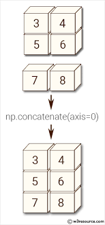
Concatenate() function can join the sequence of arrays that we provide, along with the axis specified. If the axis is not explicitly given, it is taken as 0
Concatenating arrays along row:

#Concatenating 1D array
arr1=np.array([1,2,3])
arr2=np.array([4,5,6])
arr=np.concatenate((arr1,arr2),axis=0)
print(arr)
#output : [1 2 3 4 5 6]
#Concatenating @d array along axis 0
arr1=np.array([[1,1,1],[1,1,1]])
arr2=np.array([[9,9,9,],[9,9,9]])
arr=np.concatenate((arr1,arr2),axis=0)
print(arr)
 #output : [[1 1 1]
             [1 1 1]
             [9 9 9]
            [9 9 9]]
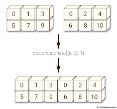
Concatenating along the column:

#concatenating along axsi 1
arr1=np.array([[1,1,1],[1,1,1]])
arr2=np.array([[9,9,9,],[9,9,9]])
arr=np.concatenate((arr1,arr2),axis=1)
print(arr)
#output : [[1 1 1 9 9 9]
           [1 1 1 9 9 9]]
Joining array using Stack function
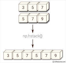
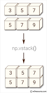
Stacking is the same as concatenation, the only difference is that stacking is done along a new axis.
np.hstack() :

#stacking two 1D arrays horizontally
arr1=np.array([0,0])
arr2=np.array([1,1])
arr=np.hstack((arr1,arr2))
# Stacking two 2D arrays horizontally
arr1=np.array([[0,0],[0,0]])
arr2=np.array([[1,1],[1,1]])
arr=np.hstack((arr1,arr2))
print(arr)
output : [[0 0 1 1]
 [0 0 1 1]]
np.vstack() :

#Stacking 1D arrays vertically
arr1=np.array([0,0])
arr2=np.array([1,1])
arr=np.vstack((arr1,arr2))
print(arr)
#output :[[0 0]
          [1 1]]
# Stacking 2D arrays vertically
arr1=np.array([[0,0],[0,0]])
arr2=np.array([[1,1],[1,1]])
arr=np.vstack((arr1,arr2))
print(arr)
#output : [[0 0]
           [0 0]
           [1 1]
           [1 1]]
Sort the arrays
sorting means simply arranging elements in an ordered sequence.
arr=np.array([3,2,0,1])
print(np.sort(arr))
#output : [0 1 2 3]
Operations on Arrays
Array Addition :
array_1 + array_2
np.array([0,1]) + np.array([2,3])
Array Subtraction
array_1 – array_2
np.array([0,1]) + np.array([2,3])
Array Multiplication
array_1 * array_2
np.array([0,1]) * np.array([2,3])
Raising by a power :
some_array ** n , where n is any real number
np.array([0,1])**2 #squaring
np.array([1,2]) ** 1.2 #raising power by 1.2
Trigonometric functions
NumPy provides the functions sin(), cos() and tan()
np.sin(some_array)
np.cos(some_array)
np.tan(some_array)
arr = np.array([1,2,3])
print( np.sin(arr) )
print( np.cos(arr) )
print( np.tan(arr) )
Exponential function :
np.exp(some_array)
np.exp(arr)
Logarithmic function :
np.log(some_array)
np.log( arr )
Applying Linear Algebra operations :
A = np.array([[6, 1, 1], [4, -2, 5], [2, 8, 7]])# Rank of a matrixprint( np.linalg.matrix_rank(A) )# Trace of matrix Aprint( np.trace(A) )# Determinant of a matrixprint(np.linalg.det(A) )# Inverse of matrix Aprint( np.linalg.inv(A) )#raising power of each elt in matrix
print(np.linalg.matrix_power(A, 3)) |
eigen_val, eigen_vec = np.linalg.eig(some_array) # to find eigen value and eigen vectors
End Notes
Thanks for reading!
We did some hands-on NumPy.I hope you enjoyed the article.
Image source links :
Image1:https://cdn.educba.com/academy/wp-content/uploads/2019/04/What-is-NumPy-1.jpg.webp
Image 2: https://www.w3resource.com/w3r_images/numpy-manipulation-concatenate-function-image-1.png
Image 3: https://www.w3resource.com/w3r_images/python-numpy-image-exercise-58.png
Image 4: https://www.w3resource.com/w3r_images/numpy-manipulation-hstack-function-image-1.png
Image 5: https://www.w3resource.com/w3r_images/numpy-manipulation-vstack-function-image-1.png


