This article was published as a part of the Data Science Blogathon
Introduction:
This article aims to explain the concepts of Natural Language Processing and how to build a model using LSTM (Long Short Term Memory), a deep learning algorithm for performing sentiment analysis. Let’s first discuss Natural Language processing!
Natural Language Processing:
Natural Language Processing (NLP) is a subfield of Artificial Intelligence that deals with understanding and deriving insights from human languages such as text and speech. Some of the common applications of NLP are Sentiment analysis, Chatbots, Language translation, voice assistance, speech recognition, etc.
Few Real-time examples:
- Google translator
- Chatbots in Apps like Flipkart & Swiggy
- Autocompletion feature in Gmail
- Personal Assistance like Alexa, Siri & Google Assistance
- Email spam detection
- Document summarization
Importance of NLP:
Why is it necessary to know about NLP? The reason for this is that in today’s world, roughly 2.5 quintillion bytes of data are generated every day. And the majority of them are inherently unstructured. Examples: Text, audio, etc. To make use of the majority of these data and to derive meaning out of it, we need to have a technology that can handle the textual and voice data. NLP is one of technology which helps to extract meaning from these types of data.
Stages in Natural Language Processing:
There are five important stages in NLP:
- Lexical Analysis
- Syntactic Analysis
- Semantic Analysis
- Discourse Integration
- Pragmatic Analysis
Lexical Analysis:
It is the first step in the NLP process where we break the texts into series of tokens or words for easy analysis. It also involves removing unnecessary blanks/white spaces from the sentences
Syntactic Analysis
This step refers to the study of how the words are arranged in a sentence to identify whether the words are in the correct order to make sense. It also involves checking whether the sentence is grammatically correct or not and converting the words to root form.
One of the common technique used in this step is:
- Stemming / Lemmatization: It is the process of converting the words to their root form. Example: Converting the word ‘Studying’ to ‘Study’. The main difference between stemming and lemmatization is stemming might not necessarily result in an actual meaningful word. But lemmatization would result in an actual meaningful word
Semantic Analysis:
This step involves looking out for the meaning of words from the dictionary and checking whether the words are meaningful.
Discourse Integration:
The meaning of a sentence in any paragraph depends on the context. Here we analyze how the presence of immediate sentences/words impacts the meaning of the next sentences/words in a paragraph.
Pragmatic Analysis:
This is the last phase of the NLP process which involves deriving insights from the textual data and understanding the context.
We got a good understanding of NLP, Let’s get into RNN and LSTM model!
Long Short Term Memory:
Before getting into LSTM, let’s understand quickly what RNN does?
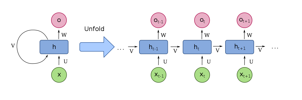
RNN is a type of supervised deep learning algorithm. Here, the neurons are connected to themselves through time. The idea behind RNN is to remember what information was there in the previous neurons so that these neurons could pass information to themselves in the future for further analysis. It means that the information from a specific time instance (t1) is used as an input for the next time instance(t2). This is the idea behind RNN.

Image source link: https://en.wikipedia.org/wiki/File:Recurrent_neural_network_unfold.svg
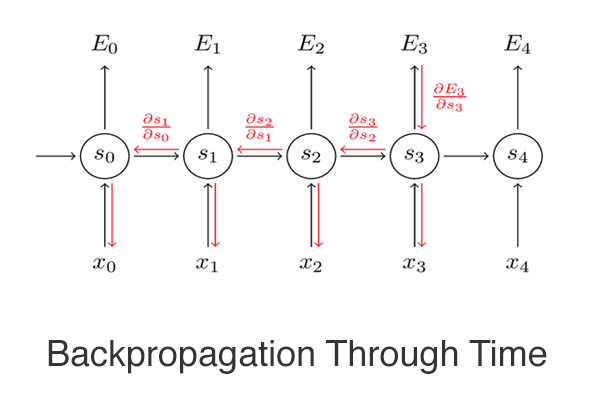
One of the major problems of RNN is the Vanishing gradient. In any neural network, the weights are updated in the training phase by calculating the error and back-propagation through the network. But in the case of RNN, it is quite complex because we need to propagate through time to these neurons.
The problem lies in calculating these weights. The gradient calculated at each time instance has to be multiplied back through the weights earlier in the network. So, as we go deep back through time in the network for calculating the weights, the gradient becomes weaker which causes the gradient to vanish. If the gradient value is very small, then it won’t contribute much to the learning process.
New weight = Old weight – (learning rate * gradient)

Image source link: https://www.techleer.com/articles/185-backpropagation-through-time-recurrent-neural-network-training-technique/
Example: Let’s say from the above diagram that we have calculated the error at time instance (t3). To update the weights of all the neurons that have participated in calculating the output at time instance(t3), we need to propagate through time till time instance (t0).
In a nutshell, if the sequence is long, then RNN finds it difficult to carry information from a particular time instance to an earlier one because of the vanishing gradient problem.
To overcome this problem, We have LSTM (Long Short Term Memory)!
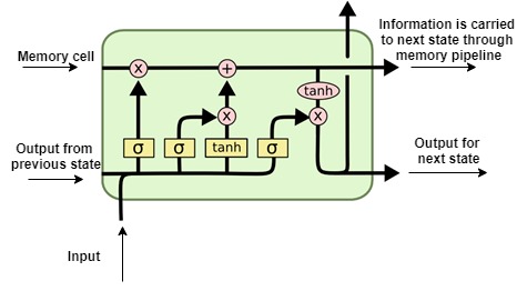
LSTM is an updated version of Recurrent Neural Network to overcome the vanishing gradient problem. Below is the architecture of LSTM with an explanation.

Image reference: https://colah.github.io/posts/2015-08-Understanding-LSTMs/
It has a memory cell at the top which helps to carry the information from a particular time instance to the next time instance in an efficient manner. So, it can able to remember a lot of information from previous states when compared to RNN and overcomes the vanishing gradient problem. Information might be added or removed from the memory cell with the help of valves.
LSTM network is fed by input data from the current time instance and output of hidden layer from the previous time instance. These two data passes through various activation functions and valves in the network before reaching the output.
Implementation of LSTM:
Now let’s get into the practical session to learn how to build an LSTM model! We will be using the Amazon Alexa products reviews dataset (link) from Kaggle.
Step 1: Importing required libraries.
# Importing required libraries
import nltk
import pandas as pd
from nltk.corpus import stopwords
from textblob import Word
from sklearn.preprocessing import LabelEncoder
from collections import Counter
import wordcloud
from sklearn.metrics import classification_report,confusion_matrix,accuracy_score
from keras.models import Sequential
from keras.preprocessing.text import Tokenizer
from keras.preprocessing.sequence import pad_sequences
from keras.layers import Dense, Embedding, LSTM, SpatialDropout1D
from sklearn.model_selection import train_test_split
import matplotlib.pyplot as plt
Step 2: Loading the dataset and creating a new column ‘sentiment’ based on ‘rating’.
Step 3: Checking for null values in the dataset.
#Check if there are any null values
data_v1 = data[['verified_reviews','sentiment']]
data_v1.isnull().sum()
Step 4: Cleaning the data. It includes removing the special characters, digits, unnecessary symbols, and stop words. Also, it is required to convert the words to their root form for easy interpretation.
def cleaning(df, stop_words):

    df['verified_reviews'] = df['verified_reviews'].apply(lambda x:

            ' '.join(x.lower() for x in x.split()))

    # Replacing the special characters

    df['verified_reviews'] = df['verified_reviews'

                                ].str.replace('[^ws]', '')

    # Replacing the digits/numbers

    df['verified_reviews'] = df['verified_reviews'].str.replace('d', ''

            )

    # Removing stop words

    df['verified_reviews'] = df['verified_reviews'].apply(lambda x:

            ' '.join(x for x in x.split() if x not in stop_words))

    # Lemmatization

    df['verified_reviews'] = df['verified_reviews'].apply(lambda x:

            ' '.join([Word(x).lemmatize() for x in x.split()]))

    return df

stop_words = stopwords.words('english')

data_v1 = cleaning(data_v1, stop_words)
Step 5: Visualizing the common words in the reviews. The size of each word represents its frequency of occurrence in the data.
common_words=''
for i in data_v1.verified_reviews:
    i = str(i)
    tokens = i.split()
    common_words += " ".join(tokens)+" "
wordcloud = wordcloud.WordCloud().generate(common_words)
plt.imshow(wordcloud, interpolation='bilinear')
plt.axis("off")
plt.show()

Step 6: Encoding the target variable using ‘Label Encoder’ from the ‘sklearn’ library.
# Encoded the target column
lb=LabelEncoder()
data_v1['sentiment'] = lb.fit_transform(data_v1['sentiment'])
Step 7: Tokenizing and converting the reviews into numerical vectors.
tokenizer = Tokenizer(num_words=500, split=' ')
tokenizer.fit_on_texts(data_v1['verified_reviews'].values)
X = tokenizer.texts_to_sequences(data['verified_reviews'].values)
X = pad_sequences(X)
- Num_words – This hyperparameter refers to the number of words to keep based on the frequency of words.
- Split – This hyperparameter refers to the separator used for splitting the word.
- pad_sequence() function is used to convert a list of sequences into a 2D NumPy array.
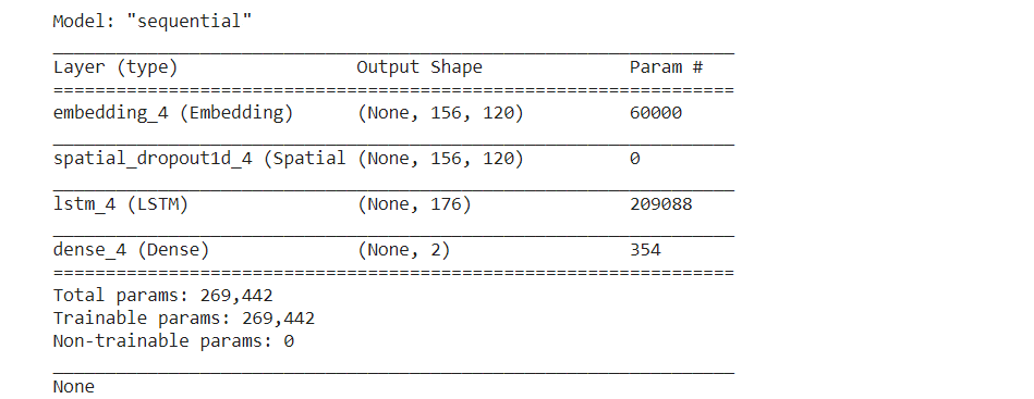
Step 8: Building the LSTM model using the ‘Keras’ library. This step involves model initialization, adding required LSTM layers, and model compilation
model = Sequential()
model.add(Embedding(500, 120, input_length = X.shape[1]))
model.add(SpatialDropout1D(0.4))
model.add(LSTM(176, dropout=0.2, recurrent_dropout=0.2))
model.add(Dense(2,activation='softmax'))
model.compile(loss = 'categorical_crossentropy', optimizer='adam', metrics = ['accuracy'])
print(model.summary())

Step 9: Splitting the data into training and testing data.
#Splitting the data into training and testing
y=pd.get_dummies(data_v1['sentiment'])
X_train, X_test, y_train, y_test = train_test_split(X,y, test_size = 0.3, random_state = 42)
Step 10: Training the model using training data.
batch_size=32
model.fit(X_train, y_train, epochs = 5, batch_size=batch_size, verbose = 'auto')

Step 11: Evaluating the model
model.evaluate(X_test,y_test)

Conclusion:
We have completed building our LSTM model for classifying the sentiments for amazon Alexa product reviews into ‘positive’ and ‘negative’ categories. The accuracy of the model is 90.9%. We can further tune the hyperparameters to improve the performance of the model.
Happy learning!
References:
- https://colah.github.io/posts/2015-08-Understanding-LSTMs/
- https://www.techleer.com/articles/185-backpropagation-through-time-recurrent-neural-network-training-technique/
About me:
I am Santhosh Kumar T, Data Analytics Intern at Empower Retirement, pursuing PGDM – Big Data Analytics at Goa Institute of Management. You can reach out to me on LinkedIn.
The media shown in this article are not owned by Analytics Vidhya and are used at the Author’s discretion.


