This article was published as a part of the Data Science Blogathon
Introduction
Do you wish you could perform this function using Pandas.
Well, there is a good possibility you can!
For data scientists who use Python as their primary programming language, the Pandas package is a must-have data analysis tool. The Pandas package has everything a data scientist needs, and every course taught us how to utilise it at first. It is so large, powerful and performs almost every tabular manipulation you can imagine. However, this breadth can be a disadvantage at times.
It has many beautiful features that solve rare edge cases, different scenarios.
One of the pandas key drawbacks is that it struggles with large datasets because pandas stores their data structures in RAM, which can become insufficient as data sizes grow. Use PySpark or Dask for this.
Even though the Pandas package is widely used, there are still many functions that people may overlook, whether because it is used less or because they are unaware of its existence. This post intends to reintroduce you to those features and demonstrate that Pandas is far more competent than you were previously aware.
Pipe

To perform data cleaning in a concise, compact manner in pandas, one can use Pipe functions, which allow you to combine multiple functions in one operation.
For example, if you like to apply functions such as drop_duplicates, encode_categoricals, remove_outliers that accept its arguments.
df_cleaned = (diamonds.pipe(drop_duplicates).
                      pipe(remove_outliers, ['price', 'carat', 'depth']).
                      pipe(encode_categoricals, ['cut', 'color', 'clarity'])
            )
Factorize
This function is an alternative to Sklearns Label Encoder.
# Mind the [0] at the end
diamonds["cut_enc"] = pd.factorize(diamonds["cut"])[0]

>>> diamonds["cut_enc"].sample(5)

52103    2
39813    0
31843    0
10675    0
6634     0
Name: cut_enc, dtype: int64
Factorize results a tuple of values: the encoded value and a list of unique categories.
values, unique = pd.factorize(diamonds["cut"], sort=True)

>>> values[:10]
array([0, 1, 3, 1, 3, 2, 2, 2, 4, 2], dtype=int64)

>>> unique
['Ideal', 'Premium', 'Very Good', 'Good', 'Fair']
Explode

Photo by Edewaa Foster on Unsplash
Explode is a function with an interesting name. Let’s start with an example and then an explanation:
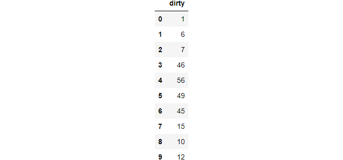
df = pd.Series([1, 6, 7, [46, 56, 49], 45, [15, 10, 12]]).to_frame("dirty")

>>> df

The feature column has two rows denoted with lists. This type of data is available in surveys where a few questions accept multiple choices.
>>> df.explode("dirty", ignore_index=True)

This function takes a cell with an array of values and explodes in multiple rows. To maintain the ordering of a numeric index, use ignore_index as True.
Between
For boolean indexing numeric features within a range, here’s a handy function:
# Get diamonds that are priced between 3500 and 3700 dollars
diamonds[diamonds["price"].between(3500, 3700, inclusive="neither")].sample(5)

T
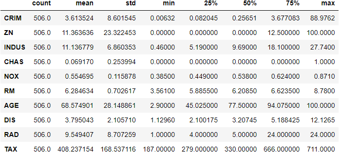
DataFrame has a simple T attribute, known as transpose. We may not use it often, describe method is helpful while viewing the dataframes.
>>> boston.describe().T.head(10)

Pandas Options
One can use global settings of pandas that helps to tweak and change the default behaviours.
>>> dir(pd.options)
['compute', 'display', 'io', 'mode', 'plotting']
It consists of 5 modules. Let’s see available options under the display. There are many options available, but I mostly use max_columns.
>>> dir(pd.options.display)

['chop_threshold',
 'max_columns',
 'max_colwidth',
 'max_info_columns',
 'max_info_rows',
 'max_rows',
 ...
 'precision',
 'show_dimensions',
 'unicode',
 'width']
Most people use max_columns and precision
# Remove the limit to display the number of cols
pd.options.display.max_columns = None

# Only show 5 numbers after the decimal
pd.options.display.precision = 5  # gets rid of scientific notation
Convert_dtypes
We’re all aware that pandas have an annoying habit of marking some columns as object data types. Rather than defining their types directly, you can use the convert dtypes method, which attempts to deduce the best data type:
sample = pd.read_csv("data/station_day.csv",usecols=["StationId", "CO", "O3", "AQI_Bucket"])

>>> sample.dtypes

StationId      object
CO            float64
O3            float64
AQI_Bucket     object
dtype: object

>>> sample.convert_dtypes().dtypes

StationId      string
CO            float64
O3            float64
AQI_Bucket     string
dtype: object
Select_dtypes
From the name, I believe it is clear what the function does. You can use the include and exclude options to specify columns that include or omit specific data types.
Choose only numeric columns with np.number, for example:
# Choose only numerical columns
diamonds.select_dtypes(include=np.number).head()

Mask

This function helps to replace values where the custom condition is not satisfied.
# Create sample data
ages = pd.Series([55, 52, 50, 66, 57, 59, 49, 60]).to_frame("ages")

ages

After performing the above operation.

Min and Max
Although min and max are well known, it has some better properties for some edge cases.
index = ["Diamonds", "Titanic", "Iris", "Heart Disease", "Loan Default"]
libraries = ["XGBoost", "CatBoost", "LightGBM", "Sklearn GB"]

df = pd.DataFrame(
    {lib: np.random.uniform(90, 100, 5) for lib in libraries}, index=index
)

>>> df

The fictional DataFrame above shows the results of four different gradient boosting libraries on five datasets. We’re looking for the package that did the best on each dataset. Here’s how to accomplish it with max in a classy manner:
>>> df.max(axis=1)

Diamonds         99.52684
Titanic          99.63650
Iris             99.10989
Heart Disease    99.31627
Loan Default     97.96728
dtype: float64
Nlargest and Nsmallest
The nlargest and nsmallest is helpful to view the top N or ~(top N) values of a variable.
diamonds.nlargest(5, "price")

diamonds.nsmallest(5, "price")

Idxmax and Idxmin
Pandas return the largest/smallest number when you call max or min on a column. However, there are situations when you need the position of the min/max, which these functions do not provide.
Instead, you can use idxmax/idxmin:
>>> diamonds.price.idxmax()
27749

>>> diamonds.carat.idxmin()
14
Value_Counts
A common way to find the percentage of the missing values is to combine isnull and sum and divide by the size of the array.
But, value_counts with relevant arguments does the same thing:
housing = pd.read_csv("train.csv")

>>> housing["FireplaceQu"].value_counts(dropna=False, normalize=True)

NaN    0.47260
Gd     0.26027
TA     0.21438
Fa     0.02260
Ex     0.01644
Po     0.01370
Name: FireplaceQu, dtype: float64
Clip

The clip function helps to find outliers outside a range and replace them with hard limits.
>>> ages.clip(50, 60)

At_time and Betweeen_time
These functions are helpful while working with time series of high granularity.
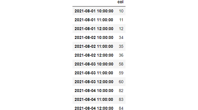
at_time helps to get values at a specific date or time.
index = pd.date_range("2021-08-01", periods=100, freq="H")
df = pd.DataFrame({"col": list(range(100))}, index=index)

>>> df.head()

>>> df.at_time(“15:00”)

between_time used to fetch rows within a custom range.
from datetime import datetime

>>> df.between_time("09:45", "12:00")

Bdate_range
This function helps to create time-series indices with business-day frequency. The financial world has this type of frequency. So, this function might be helpful at the time of reindexing time-series with reindex function.
series = pd.bdate_range("2021-01-01", "2021-01-31")  # A period of one month

>>> len(series)
21
At and Iat
These two accessors are substantially faster than loc and iloc. However, they have a drawback. They only allow you to choose or replace one value at a time:
# [index, label]
>>> diamonds.at[234, "cut"]
'Ideal'

# [index, index]
>>> diamonds.iat[1564, 4]
61.2

# Replace 16541th row of the price column
>>> diamonds.at[16541, "price"] = 10000
Argsort
This function helps to extract indices that would sort an array of the features.
tips.reset_index(inplace=True, drop=True)

sort_idx = tips["total_bill"].argsort(kind="mergesort")

# Now, sort `tips` based on total_bill
tips.iloc[sort_idx].head()

Cat Accessor
The pandas allow built-in functions of python on dates and strings using accessors like str or dt.
>>> diamonds.dtypes

carat       float64
cut        category
color      category
clarity    category
depth       float64
table       float64
price         int64
x           float64
y           float64
z           float64
cut_enc       int64
dtype: object
One can use many special functions using cat accessor on categorical columns. It has functions such as categories to find unique, rename_categories to rename the features.
diamonds["new_cuts"] = diamonds["cut"].cat.rename_categories(list("ABCDE"))

>>> diamonds["new_cuts"].cat.categories
Index(['A', 'B', 'C', 'D', 'E'], dtype='object')
Check this out for a more list of functions under cat accessor.
Squeeze
Squeeze is a function used in rare yet aggravating edge circumstances.
When a single value is returned from a condition used to subset a DataFrame, this is one of these cases. Consider the following scenario:
subset = diamonds.loc[diamonds.index >> subset

Even if there is only one cell, return the DataFrame. It is inconvenient since you must now use.loc with both the column name and index to obtain the price.
You don’t have to if you know how to squeeze. An axis can be removed from a single-cell DataFrame or Series using this function. Consider the following scenario:
>>> subset.squeeze()
326
It is possible to specify the axis to remove. It had only returned scalar now.
>>> subset.squeeze("columns")  # or "rows"

0    326
Name: price, dtype: int64
Note this function only works for Series or DataFrame with single values.
Excel_writer
It is a generic class for creating excel files and writing DataFrame in it. Consider, we have these two datasets.
# Load two datasets
diamonds = sns.load_dataset("diamonds")
tips = sns.load_dataset("tips")

# Write to the same excel file
with pd.ExcelWriter("data/data.xlsx") as writer:

    diamonds.to_excel(writer, sheet_name="diamonds")
    tips.to_excel(writer, sheet_name="tips")
It has properties to specify the DateTime format to use, whether you need a new file or modify an existing one, what happens if a sheet exists. Check this documentation for more details.
Conclusion
It is not an exhaustive overview of pandas, and the documentation contains more information on the code and features. I recommend that you experiment with different variations of the code snippets provided here, as well as various parameters. One can fully comprehend the power of pandas by doing this.
Libraries like Dask and datatable are gradually displacing Pandas with their flashy new features for handling large datasets, Pandas remains the most extensively used data manipulation tool in the Python data science community. Because of how well it fits into the present SciPy stack, the library serves as a paradigm for other packages to follow and build.
I hope you had found this post insightful and thank you for reading.


