This article was published as a part of the Data Science Blogathon.
Introduction
Handwritten digit classification is one of the multiclass classification problem statements. In this article, we’ll introduce the multiclass classification using Support Vector Machines (SVM). We’ll first see what exactly is meant by multiclass classification, and we’ll discuss how SVM is applied for the multiclass classification problem. Finally, we’ll look at Python code for multiclass classification using Sklearn SVM.
The particular question on which we will be focusing in this article is as follows:
“How can you extend a binary classifier to a multi-class classifier in case of SVM algorithm?”
Multiclass Classification: In this type of classification, the machine learning model should classify an instance as only one of three classes or more. For Example, Classifying a text as positive, negative, or neutral.
Let’s get started,
What are Support Vector Machines (SVM)?
SVM is a supervised machine learning algorithm that helps in both classification and regression problem statements. It tries to find an optimal boundary (known as hyperplane) between different classes. In simple words, SVM does complex data transformations depending on the selected kernel function, and based on those transformations, it aims to maximize the separation boundaries between your data points.
Working of SVM:
In the simplest form where there is a linear separation, SVM tries to find a line that maximizes the separation between a two-class data set of 2-dimensional space points.
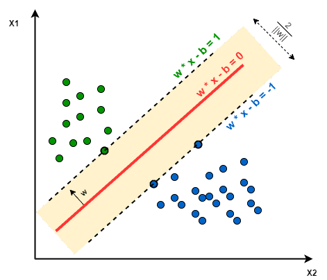
The objective of SVM: The objective of SVM is to find a hyperplane that maximizes the separation of the data points to their actual classes in an n-dimensional space. The data points which are at the minimum distance to the hyperplane i.e, closest points are called Support Vectors.
For Example, For the given diagram, the three points that are layered on the scattered lines are the Support Vectors (2 blue and 1 green), and the separation hyperplane is the solid red line.
Fig. Image showing the Support Vectors
Image Source: link
Multiclass Classification Using SVM
In its most basic type, SVM doesn’t support multiclass classification. For multiclass classification, the same principle is utilized after breaking down the multi-classification problem into smaller subproblems, all of which are binary classification problems.
The popular methods which are used to perform multi-classification on the problem statements using SVM are as follows:
👉 One vs One (OVO) approach
👉 One vs All (OVA) approach
👉 Directed Acyclic Graph (DAG) approach
Now, let’s discuss each of these approaches one by one in a detailed manner:
One vs One (OVO)
👉 This technique breaks down our multiclass classification problem into subproblems which are binary classification problems. So, after this strategy, we get binary classifiers per each pair of classes. For final prediction for any input use the concept of majority voting along with the distance from the margin as its confidence criterion.
👉 The major problem with this approach is that we have to train too many SVMs.
👉 Let’s have Multi-class/ Multi-labels problems with L categories, then:
For the (s, t)- th classifier:
– Positive Samples: all the points in class s ({ xi : s ∈ yi })
– Negative samples: all the points in class t ({ xi : t ∈ yi })
– fs, t(x): the decision value of this classifier
( large value of f s, t(x) ⇒ label s has a higher probability than the label t )
– f t, s (x) = – f s, t(x)
– Prediction: f(x)= argmax s ( Σ t fs, t(x) )
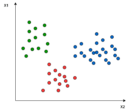
👉 Let’s have an example of 3 class classification problem: Green, Red, and Blue.
Fig. Image showing 3 different classes
Image Source: link
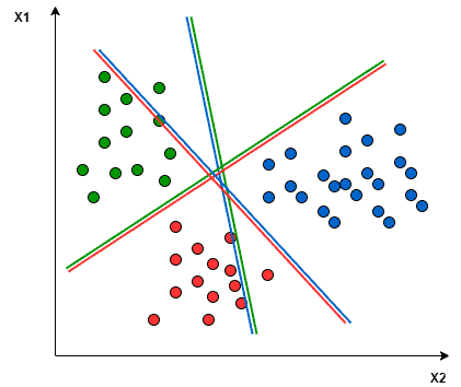
👉 In the One-to-One approach, we try to find the hyperplane that separates between every two classes, neglecting the points of the third class.
For example, here Red-Blue line tries to maximize the separation only between blue and red points while It has nothing to do with the green points.
Fig. One vs One Approach
Image Source: link
One vs All (OVA)
👉 In this technique, if we have N class problem, then we learn N SVMs:
SVM number -1 learns “class_output = 1” vs “class_output ≠ 1″
SVM number -2 learns “class_output = 2” vs “class_output ≠ 2″
:
SVM number -N learns “class_output = N” vs “class_output ≠ N”
Then to predict the output for new input, just predict with each of the build SVMs and then find which one puts the prediction the farthest into the positive region (behaves as a confidence criterion for a particular SVM).
👉 Now, a very important comes to mind that “Are there any challenges in training these N SVMs?”
Yes, there are some challenges to train these N SVMs, which are:
1. Too much Computation: To implement the OVA strategy, we require more training points which increases our computation.
2. Problems becomes Unbalanced: Let’s you are working on an MNIST dataset, in which there are 10 classes from 0 to 9 and if we have 1000 points per class, then for any one of the SVM having two classes, one class will have 9000 points and other will have only 1000 data points, so our problem becomes unbalanced.
Now, how to address this unbalanced problem?
You have to take some representative (subsample) from the class which is having more training samples i.e, majority class. You can do this by using some below-listed techniques:
– Use the 3-sigma rule of the normal distribution: Fit data to a normal distribution and then subsampled accordingly so that class distribution is maintained.
– Pick some data points randomly from the majority class.
– Use a popular subsampling technique named SMOTE.
👉 Let’s have Multi-class/ multi-labels problems with L categories, then:
For the t -th classifier:
– Positive Samples: all the points in class t ({ xi : t ∈ yi })
– Negative samples: all the points not in class t ({ xi : t ∉ yi })
– ft(x): the decision value for the t -th classifier.
( large value of ft ⇒ higher probability that x is in the class t)
– Prediction: f(x) = argmax t ft(x)
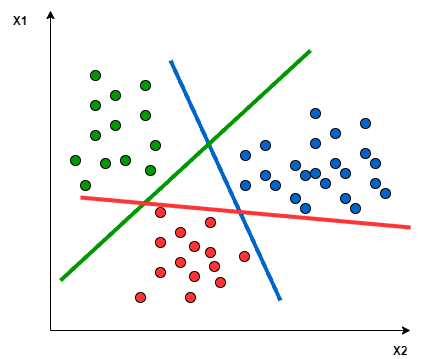
👉 In the One vs All approach, we try to find a hyperplane to separate the classes. This means the separation takes all points into account and then divides them into two groups in which there is a group for the one class points and the other group for all other points.
For example, here, the Greenline tries to maximize the gap between green points and all other points at once.
Fig. One vs All approach
Image Source: link
NOTE: A single SVM does binary classification and can differentiate between two classes. So according to the two above approaches, to classify the data points from L classes data set:
👉 In the One vs All approach, the classifier can use L SVMs.
👉 In the One vs One approach, the classifier can use L(L-1)/2 SVMs.
Directed Acyclic Graph (DAG)
👉 This approach is more hierarchical in nature and it tries to addresses the problems of the One vs One and One vs All approach.
👉 This is a graphical approach in which we group the classes based on some logical grouping.
👉 Benefits: Benefits of this approach includes a fewer number of SVM trains with respect to the OVA approach and it reduces the diversity from the majority class which is a problem of the OVA approach.
👉 Problem: If we have given the dataset itself in the form of different groups ( e.g, cifar 10 image classification dataset ) then we can directly apply this approach but if we don’t give the groups, then the problem with this approach is of finding the logical grouping in the dataset i.e, we have to manually pick the logical grouping.
End Notes
Thanks for reading!
If you liked this and want to know more, go visit my other articles on Data Science and Machine Learning by clicking on the Link
Please feel free to contact me on Linkedin, Email.
Something not mentioned or want to share your thoughts? Feel free to comment below And I’ll get back to you.
About the author
Chirag Goyal
Currently, I am pursuing my Bachelor of Technology (B.Tech) in Computer Science and Engineering from the Indian Institute of Technology Jodhpur(IITJ). I am very enthusiastic about Machine learning, Deep Learning, and Artificial Intelligence.
The media shown in this article are not owned by Analytics Vidhya and is used at the Author’s discretion.


