Introduction
When I started learning about machine learning just for the sake of interest I thought ML is something only people in the IT field should learn and have scope to implement, but when I actually started deep diving into various ML techniques I found that in near future there will be hardly any field which will not use ML or AI. Let us consider an example in the field of building automation.
The big advantage of machine learning is that it is not limited to explicit programming; it can monitor all equipment systems in a building and detect anomalies that could not possibly have been programmed ahead of time by humans. Let us consider one simple basic example of predicting heating and cooling load i.e. energy efficiency of the building using some building features. I have used the energy efficiency dataset from the UCI Machine learning repository.
We will implement an artificial neural network model for this task using R as a programming language. Following are the basic steps while applying any machine learning algorithm to any dataset.
- Exploratory Data Analysis (EDA)
- Outlier and missing value treatment
- Dummy variable creation (if applicable)
- Data normalization (if applicable)
- Test and train dataset preparation
- Model building
- Model performance evaluation
- Conclusion
Now let us explore these steps in detail for our example. Here is a brief look at variables available in the dataset.
- X2: Surface Area
- X3: Wall Area
- X4: Roof Area
- X5: Overall Height
- X6: Orientation
- X7: Glazing Area
- X8: Glazing Area Distribution
- Y1: Heating Load
- Y2: Cooling Load
The first step in this process is to explore given data (EDA). Here variables X1 to X7 are predictors (Independent variables) and Y1 and Y2 are dependent (target variables). Now we will read the dataset using the read_excel command and explore the variables individually using the summarytool package. Also, we can check the correlation matrix for the variables as a part of EDA.
library(readxl)
mydata=read_excel("ENB2012_data.xlsx", sheet = "Data")
install.packages("summarytools")
library(summarytools)
summarytools::view(dfSummary(mydata))
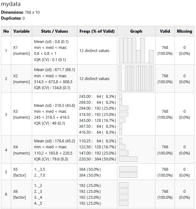
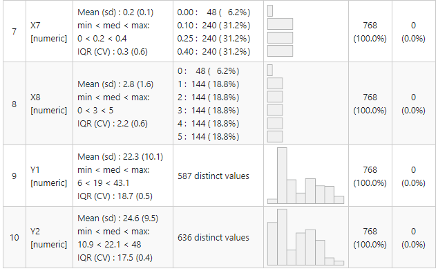
The summary tool package gives you results in the below format. Isn’t cool to have 5 point summary, missing value, duplicate value, variable distribution all in one place.
install.packages("summarytools")
library(summarytools)
summarytools::view(dfSummary(mydata))


Looking at the last column of the table we observe that the dataset has no missing values.
All variables are identified as numeric by R, but we observe that variable X5 (Overall Height) has two only two values 3.5 and 7.0 also variable X6 (Orientation) has only 4 values so we define them as factors with 2 and 4 levels respectively.
mydata$X5=as.factor(mydata$X5)
levels(mydata$X5)=c("_3.5", "_7.0")
mydata$X6=as.factor(mydata$X6)
levels(mydata$X5)=c("_2", "_3","_4", "_5")
Before actually building the ANN model another important step is dummy variables creation as the ANN model does not accept categorical variables. A dummy variable is a numerical variable used to represent subgroups of the sample in our study. Now we convert X5 and X6 to dummy variables, and consider 1 dummy variable for X5 and 3 dummy variables for X6, as a general rule is to use one fewer dummy variable than categories.
library(dummies)
View(mydata)
mydata=data.frame(mydata)
data=dummy.data.frame(mydata, names=c("X5", "X6"))
Now we divide the dataset into a 70:30 ratio, naming it as train and test dataset. Train dataset we use to train our model and test dataset we use for predict values using trained model.
As ANN is a weight-based algorithm, Normalization is required so that all the inputs are at a comparable range and will get unbiased output. Among the best practices for training a Neural Network is to normalize your data to obtain a mean close to 0. Normalizing the data generally speeds up learning and leads to faster convergence. We take out output variables from the dataset before normalizing predictors.
train=data[1:537,]
test=data[538:768,]
train1=train[,-c(13,14)]
test1=test[,-c(13,14)]
train_sc = scale(train1)
library(caret)
train_scale = preProcess(train1)
test_sc= predict(train_scale, test1)
train_sc=cbind(train[,13:14],train_sc)
test_sc=cbind(test[,13:14], test_sc)
Now the training dataset is ready to build our artificial neural network model. Artificial Neural Network (ANN) uses the processing of the brain as a basis to develop algorithms that can be used to model complex patterns and prediction problems.
Three main reasons why we selected ANN here is:
1. ANNs have the ability to learn and model non-linear and complex relationships, which is really important because, in real life, many of the relationships between inputs and outputs are non-linear as well as complex.
2. ANNs can generalize — After learning from the initial inputs and their relationships, they can infer unseen relationships on unseen data as well, thus making the model generalize and predict on unseen data.
3. Unlike many other prediction techniques, ANN does not impose any restrictions on the input variables (like how they should be distributed).
Here we implement ANN using “neuralnet” package in r.
library(neuralnet)
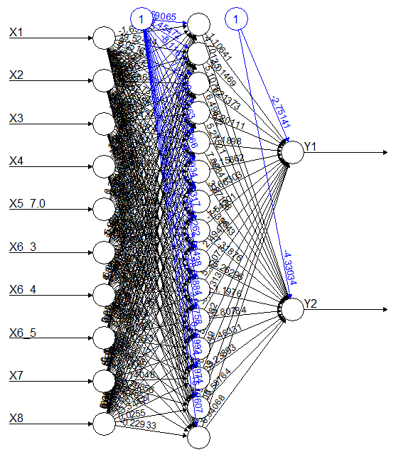
NN_model = neuralnet(Y1 +Y2 ~ X1+X2+X3+X4+X5_7.0+X6_3+X6_4++X6_5+X7+X8, data= train_sc, hidden = 15,linear.output = TRUE, stepmax =1e+06,rep=1, lifesign.step = 1000, threshold = 0.5 )
plot(NN_model)

Here you may need to play around parameters like stepmax, no. of repetitions, and no. of hidden layers unless we get which converge and gives less value of mean square error (MSE) for predicted values. Using this model we now predict values of Y1 and Y2 of train and test datasets.
train$pred_Y1=NN_model$net.result[[1]][,1]
library(MLmetrics)
mse=MSE(train$pred_Y1, train$Y1)
train$pred_Y2=NN_model$net.result[[1]][,2]
mse=MSE(train$pred_Y2, train$Y2)
model_results=compute(NN_model,test_sc[3:14])
test$pred_Y1=model_results$net.result[,1]
test$pred_Y2=model_results$net.result[,2]
cor(test$pred_Y1,test$Y1)
cor(test$pred_Y2,test$Y2)
Here we get MSE of 0.35 and 0.9072 for the train dataset and 1.7 and 1.5 for the test dataset. We look at the correlation coefficient of actual and predicted values which comes in the range of 0.97 to 0.99 indicating that predicted values are closely following actual values. Thus our model is doing well for this dataset.
We can also implement a linear regression model for the same and compare its performance with this model and use the best-fitted model for further HVAC system design. If you have read so far surely you would like to try your hands-on ML implementation in your field.
The media shown in this article on Building Automation are not owned by Analytics Vidhya and is used at the Author’s discretion.


