This article was published as a part of the Data Science Blogathon.
Introduction
Will tomorrow be a sunny day? What are the chances that a student will get into that dream university? These and many more real-world “decision” scenarios need a standard mechanism. Step in Logistic Regression may be stated very simply as an estimation of the probability of an event occurring. In the next few minutes, we shall understand Logistic Regression from A-to-Z. We will first implement it using MS Excel and then Python (using packages like sklearn and statsmodel) to obtain regression coefficients. This should help reinforce and ensure a holistic understanding of the concept. We conclude by interpreting the chosen regression coefficient in terms of the odds ratio. Of course, we will need a dataset to work with, so let’s get it out of the way first and then focus on the subject matter.
About the dataset
I have created a dummy dataset for this implementation, much smaller than anything you encounter in the wild. Our dataset deals with Common Entrance Test (CET) scores and determines whether a student will succeed in getting admission to the university or not. For this, the dataset has one ‘independent’ or ‘predictor’ variable: the Common Entrance Test (CET) score and a ‘dependent’ or ‘response’ variable (whether the student makes the cut or not, whether they get in or not). Our problem statement is, of course, to predict whether the student can get into a university given their CET score.
About Logistic Regression
The target variable is discrete in logistic regression (unlike linear regression). It is a supervised machine learning algorithm used to address classification problems. Output from a logistic regression implementation is the estimate of the probability of a particular event occurring. As Probability goes, it is always in the range of 0 to 1.
Understanding the odds ratio
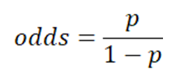
If the Probability of a particular event occurring is p, then the probability of that event not occurring is (1-p). The ratio of p to (1-p) is called the Odds, as follows-
In simple linear regression, the model to estimate the continuous response variable y as a linear function of the explanatory variable x as follows-
However, when the response variable is discrete, in terms of 1 or 0 (True or False, Success or Failure), estimation is done based on the Probability of success. Logistic regression classifier models the estimate of probability p in terms of the predictor or explanatory variables x. The natural log of odds or the logit function is used for this transformation. For a single predictor variable, the transformation equation is given as follows-
Estimate of Probability can also be written in terms of sigmoid function as-.
Logistic Regression – The MS Excel Way
Watch the video explaining obtaining Logistic Regression coefficients in MS Excel.
Logistic Regression – The Python Way
To do this, we shall first explore our dataset using Exploratory Data Analysis (EDA) and then implement logistic regression and finally interpret the odds:
1. Import required libraries
2. Load the data, visualize and explore it
3. Clean the data
4. Deal with any outliers
5. Split the data into a training set and testing set
6. Fit a logistic regression model using sklearn
7. Apply the model on the test data and make a prediction
8. Evaluate the model accuracy using the confusion matrix
9. Create the model and obtain the regression coefficients using statsmodel
10. the essential thing is, Interpret the regression coefficient in terms of the odds
Step 1- Import required libraries
Here the built-in sklearn packages for splitting data into training and test sets and implementing logistic regression are used. confusion_matrix and accuracy_score functions are used to evaluate the model. A confusion matrix is visualized using a heatmap from the seaborn package, and Boxplot from seaborn is used to check for the outliers in the dataset.
#import the relevant libraries
import numpy as np
import matplotlib.pyplot as plt
import pandas as pd
import seaborn as sns
from sklearn.linear_model import LogisticRegression
from sklearn.model_selection import train_test_split
from sklearn.metrics import confusion_matrix, accuracy_score
%matplotlib inline
import warnings #to remove the warnings
warnings.filterwarnings('ignore')
Step 2- Load, visualize and explore the dataset
df= pd.read_csv('/content/CET_logistics_1.csv') #read the dataset
#Explore the dataset
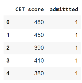
df.head()
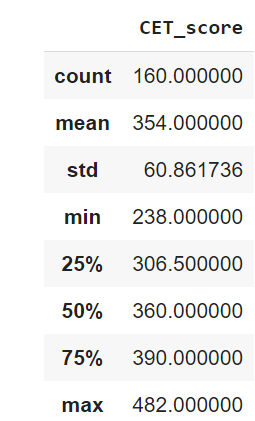
df.describe() #To know more about the dataset
Step 3- Clean the data set
From the output of described method, it is understood that the CET_score column does not have any zeros. However, we need to check if there are any null entries in the columns for the data frame. This can be done as follows-
#Check for null entries
print("Number of null values in the data set are - ",df.isnull().values.any().sum())
It is understood that there are no null values also in the dataset. However, it is observed that the target column “admitted” column has non-numerical values “Yes and “No”. So these are replaced for numbers 1 and 0 respectively.
#Replace yes and no entries in target to 1 and 0 repsectively
df=df.replace({'admittted':{'Yes':1, 'No':0}})
Step 4- Deal with the outliers
The following code is implemented to check any outliers in the predictor variables.
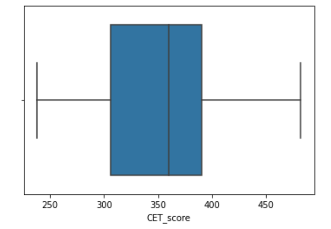
From the boxplot, it is seen that there are no outliers below the 25th percentile and above the 75th percentile. So there is no need to remove any outliers. However, if the outliers are to be removed, the following function can be used.
#Function to find the upper and lower limits to identify and remover outliers
def interQuartile(x):
  percentile25= x.quantile(0.25)
  percentile75=x.quantile(0.75)
  iqr=percentile75-percentile25
  upperLimit= percentile75+1.5*iqr
  lowerLimit= percentile25-1.5*iqr
  return upperLimit, lowerLimit
"""
To find the upper and lower limit CET_score column and
check if any values are beyond these limits
"""
upper,lower= interQuartile(df['CET_score'])
print("Lower and upper limit calculated are -", upper, lower)
#To print the number of datapoints below and above these limits
print("Number of entries below the lower limit are ", (df['CET_score'] < lower).sum())
print("Number of entries above the upper limit are ", (df['CET_score'] > upper).sum())
Step 5: Define dependent and independent variables and then split the data into a training set and testing set.
In this step, the independent and dependent variables are first defined, and then the data set is split into training and testing data. A ratio of 80-20 is used in this implementation for training and testing, respectively.
#Define the independent and dependent variables
y= df['admittted'] #dependent variable is Decision
x= df.drop(['admittted'], axis=1)
# splitting the data
x_train, x_test, y_train, y_test = train_test_split(x,y, test_size= 0.2)
Step 6- Fit a logistic regression model using sklearn
In this step, a logistic regression classifier is created, and the model is fitted with the help of the training data to obtain the regression coefficients.
#Implementing Logistic Regression using sklearn
modelLogistic = LogisticRegression()
modelLogistic.fit(x_train,y_train)
#print the regression coefficients

print("The intercept b0= ", modelLogistic.intercept_)

print("The coefficient b1= ", modelLogistic.coef_)
Regression coefficients obtained are b0= -68.8307661 and b1=0.19267811
Step 7- Apply the model on the test data and make a prediction
The following code is used to obtain the predicted values for the test data.
#Make prediction for the test data
y_pred= modelLogistic.predict(x_test)
Step 8- Evaluate the model using a confusion matrix to obtain an accuracy rate.
The confusion matrix consists of the matrix elements with True Positive, True Negative, False Positive, and False Negative values. It can be obtained using the code below, and these terms can be explained with the help of the confusion matrix plotted.
#Creating confusion matrix
ConfusionMatrix = confusion_matrix(y_test, y_pred)
print(ConfusionMatrix)
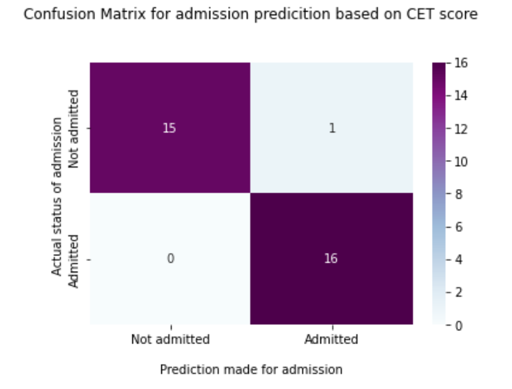
True Positive- The number of predictions made for admission is “Admitted,” and the actual status of the entry is also “Admitted”. In this case, True Positive= 16.
True Negative- The number of predictions made for admissions is “Not Admitted,” and the actual status of the entrance is also “Not admitted.”
Similarly, False Positive is several predictions made for “Admitted” when the status was “Not admitted”. Here the False Positive = 1.
False Negative can be obtained similarly.
Now accuracy is given by several true predictions divided by the total number of predictions made. From the above confusion matrix, accuracy rate =31/32= 0.96875.
Following code can be used to obtain the accuracy rate-
#Accuracy from confusion matrix
TP= ConfusionMatrix[1,1] #True positive
TN= ConfusionMatrix[0,0] #True negative
Total=len(y_test)
print("Accuracy from confusion matrix is ", (TN+TP)/Total)
Step 9: Obtain the regression coefficients using the statsmodel package
#Using statsmodels package to obtian the model
import statsmodels.api as sm
x_train = sm.add_constant(x_train)
logit_model=sm.Logit(y_train,x_train)
result=logit_model.fit()
print(result.summary())
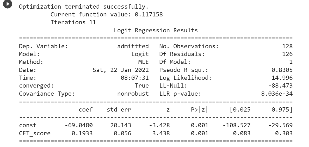
It is seen from the figure that the same values of the regression coefficients are obtained.
Step 10: Interpreting the value of coefficient b1 in terms of odds ratio
Let us calculate the log of odds for CET_Score= 372 and 373.
ln(Odds(372))= b0+b1*372= -69.048+0.1933*372= 2.8596

ln(Odds(373)= b0+b1*373=-69.048+0.1933*373=3.0529

Now taking difference of both the odds,

ln(Odds(373)) - ln(Odds(372)) = 3.0529-2.8596= 0.1933=b1

Therefore the Odd Ratio is

ln(Odds(373)/Odds(372))= b1

Takin antilog on both the sides,

Odds(373)/Odds(372)= e^b1

Odds(373)/Odds(372)= e^0.1933

Odds(373)/Odds(372)= 1.2132
Therefore, for everyone mark increase in the CET score, the odds increase by 21.3%.
Let us take one more example where we want to compare in terms of odd ratio candidate A with 340 marks to candidate B with 355 marks.
Odds Ratio= Odds(355)/Odds(340)= e^(355-340)b1= e^15b1= 18.165.
So we can say that odds of getting admission for candidate B are approximately 18 times more than candidate A.
Summary
In this article, we have seen the step-by-step implementation of logistic regression with one independent variable in excel and Python. Along with the basic understanding of the mathematical concept, we have also seen how to interpret the regression coefficient in terms of the odds ratio.
Read more articles on Logistic Regression on our blog.
The media shown in this article is not owned by Analytics Vidhya and are used at the Author’s discretion.


