This article was published as a part of the Data Science Blogathon.
Introduction
As a data scientist, in many cases of fraud detection in the bank for a transaction, Smart meters anomaly detection, how will you identify anomalies or outliers?
A data point significantly off the average and, depending on the goal, either removing or resolving them from the analysis to prevent skewing is known as outlier detection.
Have you ever thought about the bank where you make several transactions and how the bank helps you by identifying fraud?
Someone logins to your account, and a message is sent to you immediately after they notice suspicious activity at a place to confirm if it’s you or someone else.
What is Anomaly Detection?
We often see the dataset having anomalies or outliers, usually defined by having different values than another dataset.
Suppose we own a company and notice the font end data errors, even when our company supplies the same service, but the sales are declining. Here come the errors, which are termed anomalies or outliers.
Let’s take an example that will further clarify what anomaly means.

Here in this example, a bird is an outlier or noise.
Have you ever thought about the bank where you make several transactions, How the bank helps you by identifying fraud detection?
If the bank manager notices unusual behavior in your accounts, it can block the card. For example, spending a lot of amount in one day or another sum amount on another day will send a message of alert or will block your card as it’s not related to how you were spending previously.
Two AI firms detect an anomaly inside the bank. One is Fedzai’s detection firm, and another one by Ayasdi’s solution.
Let’s take another example of shopping, at the end of the month, the shopkeeper puts certain items on sale and offers you a scheme where you can buy two at less rate.
Now how do we describe the sales data compared to the start-of-month data? Do sale data validate data concerning monthly sales at the start of selling? It’s not valid data is noise.
Outliers are “something I should remove from the dataset so that it doesn’t skew the model I’m building,” typically because they suspect that the data in question is flawed and that the model they want to construct shouldn’t need to take into account.
Outliers are most commonly caused by:
Intentional (dummy outliers created to test detection methods)
Data processing errors (data manipulation or data set unintended mutations)
Sampling errors (extracting or mixing data from wrong or various sources)
Natural (not an error, novelties in the data)
Data entry errors (human errors)
Difference Between Anomaly and Outlier
An actual data point significantly outside a distribution’s mean or median is an outlier.
An anomaly is a false data point made by a different process than the rest of the data.
If you construct a linear regression model, it is less likely that the model generated points far from the regression line. The likelihood of the data is another name for it.
Outliers are data points with a low likelihood, according to your model. They are identical from the perspective of modeling.
For instance, you could construct a model that describes a trend in the data and then actively looks for existing or new values with a very low likelihood. When people say “anomalies,” they mean these things. The anomaly detection of one person is the outlier of another!
Extreme values in your data series are called outliers. They are questionable. One student can be much more brilliant than other students in the same class, and it is possible.
However, anomalies are unquestionably errors. For example, one million degrees outside, or the air temperature won’t stay the same for two weeks. As a result, you disregard this data.
How will you differentiate outlier and noise data?
An outlier is a valid data point, and can’t be ignored or removed, whereas noise is garbage that needs removal. Let’s take another example to understand noise.
Suppose you wanted to take the average salary of employees and in data added the pay of Ratan Tata or Bill Gate, all the employer’s salary averages will show an increase which is incorrect data.
Detection of anomalies can lead to fraud detection, improve your data, and leads to correct data analysis.
1. Outlier – Outliers are extreme data points that go above and beyond what is typical of their kind. That could be a particular data set or a whole data set.
2. Uni-variate – Uni-variate a variable with different values in the dataset.
3. Multi-variate – It is defined by the dataset by having more than one variable with a different set of values.
We will now use various techniques which will help us to find outliers.
Anomaly Detection by Scikit-learn
We will take a simple Titanic dataset from the link, The Complete Titanic Dataset | Kaggle, and run it on Jupyter notebook.
We will import the required library and read our data.
import seaborn as sns
import pandas as pd
titanic=pd.read_csv('titanic.csv')
titanic.head()

We can see in the image many null values. We will fill the null values with mode.
titanic['age'].fillna(titanic['age'].mode()[0], inplace=True)
titanic['cabin'].fillna(titanic['cabin'].mode()[0], inplace=True)
titanic['boat'].fillna(titanic['boat'].mode()[0], inplace=True)
titanic['body'].fillna(titanic['body'].mode()[0], inplace=True)
titanic['sex'].fillna(titanic['sex'].mode()[0], inplace=True)
titanic['survived'].fillna(titanic['survived'].mode()[0], inplace=True)
titanic['home.dest'].fillna(titanic['home.dest'].mode()[0], inplace=True)
Let’s see our data in more detail. When we look at our data in statistics, we prefer to know its distribution types, whether binomial or other distributions.
titanic['age'].plot.hist(
  bins = 50,
  title = "Histogram of the age"
)
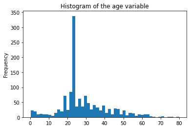
This distribution is Gaussian distribution and is often called a normal distribution.
Mean and Standard Deviation are considered the two parameters. With the change in mean values, the distribution curve changes to left or right depending on the mean values.
Standard Normal distribution means mean(μ = 0) and standard deviation (σ) is one. To know the probability Z-table is already available.
Z-Scores
We can calculate Z – Scores by the given formula where x is a random variable, μ is the mean, and σ is the standard deviation.
Why do we need Z-Scores to be calculated?
It helps to know how a single or individual value lies in the entire distribution.
For example, if the maths subject scores mean is given to us 82, the standard deviation σ is 4. We have a value of x as 75. Now Z-Scores will be calculated as 82-75/4 = 1.75. It shows the value 75 with a z-score of 1.75 lies below the mean. It helps to determine whether values are higher, lower, or equal to the mean and how far.
Now, we will calculate Z-Score in python and look at outliers.
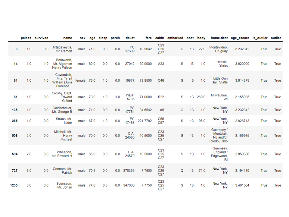
We imported Z-Scores from Scipy. We calculated Z-Score and then filtered the data by applying lambda. It gives us the number of outliers ranging from the age of 66 to 80.
from scipy.stats import zscore
titanic["age_zscore"] = zscore(titanic["age"])
titanic["outlier"] = titanic["age_zscore"].apply(
  lambda x: x = 2.8
)
titanic[titanic["outlier"]]
We will now look at another method based on clustering called Density-based spatial clustering of applications with noise (DBSCAN).
DBSCAN
As the name indicates, the outliers detection is on clustering. In this method, we calculate the distance between points.
Let’s continue our titanic data and plot a graph between fare and age. We made a scatter graph between age and fare variables. We found three dots far away from the others.
Before we proceed further, we will normalize our data variables.
There are many ways to make our data normalize. We can import standard scaler by sklearn or min max scaler.
titanic['fare'].fillna(titanic['fare'].mean(), inplace=True)
from sklearn.preprocessing import StandardScaler
scale = StandardScaler()
fage = scale.fit_transform(fage)
fage = pd.DataFrame(fage, columns = ["age", "fare"])
fage.plot.scatter(x = "age", y = "fare")
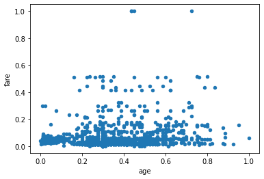
We used Standard Scaler to make our data normal and plotted a scatter graph.
Now we will import DBSCAN to give points to the clusters. If it fails, it will show -1.
from sklearn.cluster import DBSCAN
outlier = DBSCAN(
  eps = 0.5,
  metric="euclidean",
  min_samples = 3,
  n_jobs = -1)
clusters = outlier.fit_predict(fage)
clusters
array([0, 1, 1, ..., 1, 1, 1])
Now we have the results, but how do we check which value is min, max and whether we have -1 values? We will use the arg min value to check the smallest value in the cluster.
value=-1
index = clusters.argmin()
print(" The element is at ", index)
small_num = np.min(clusters)
print("The small number is : " , small_num)
print(np.where(clusters == small_num))
The element is at: 14
The small number is : -1
(array([ 14, 50, 66, 94, 285, 286], dtype=int64),)
We can see from the result six values which are -1.
Lets now plot a scatter graph.
from matplotlib import cm
c = cm.get_cmap('magma_r')
fage.plot.scatter(
  x = "age",
  y = "fare",
  c = clusters,
  cmap = c,
  colorbar = True
)
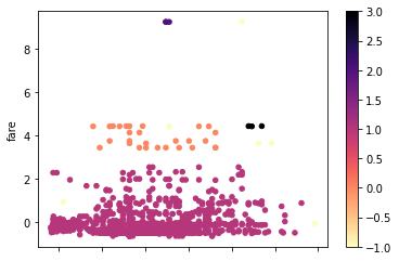
The above methods we applied are on uni-variate outliers.
For Multi-variates outliers detections, we need to understand the multi-variate outliers.
For example, we take Car readings. We have seen two reading meters one for the odometer, which records or measures the speed at which the vehicle is moving, and the second is the rpm reading which records the number of rotations made by the car wheel per minute.
Suppose the odometer shows in the range of 0-60 mph and rpm in 0-750. We assume that all the values which come should correlate with each other. If the odometer shows a 50 speed and the rpm shows 0 intakes, readings are incorrect. If the odometer shows a value more than zero, that means the car was moving, so the rpm should have higher values, but in our case, it shows a 0 value. i.e., Multi-variate outliers.
Mahalanobis Distance Method
In DBSCAN, we used euclidean distance metrics, but in this case, we are talking about the Mahalanobis distance method. We can also use Mahalanobis distance with DBSCAN.
DBSCAN(eps=0.5, min_samples=3, metric='mahalanobis', metric_params={'V':np.cov(X)}, algorithm='brute', leaf_size=30, n_jobs=-1)Why is Euclidean unfit for entities cor-related to each other? Euclidean distance cannot find or will give incorrect data on how close are the two points.
Mahalanobis method uses the distance between points and distribution that is clean data. Euclidean distance is often between two points, and its z-score is calculated by x minus mean and divided by standard deviation. In Mahalanobis, the z-score is x minus the mean divided by the covariance matrix.
Therefore, what effect does dividing by the covariance matrix have? The covariance values will be high if the variables in your dataset are highly correlated.
Similarly, if the covariance values are low, the distance is not significantly reduced if the data are not correlated. It does so well that it addresses both the scale and correlation of the variables issues.
Code
Dataset can be taken from Anomaly-/caret.csv at main · aster28/Anomaly- (github.com)
df = pd.read_csv('caret.csv').iloc[:, [0,4,6]]
df.head()
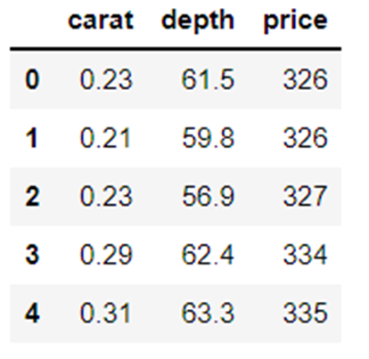
We defined the function distance as x= None, data= None, and Covariance = None. Inside the function, we took the mean of data and used the covariance value of the value there. Otherwise, we will calculate the covariance matrix. T stands for transpose.
For example, if the array size is five or six and you want it to be in two variables, then we need to transpose the matrix.
np.random.multivariate_normal(mean, cov, size = 5)
array([[ 0.0509196,  0.536808 ],
       [ 0.1081547,  0.9308906],
       [ 0.4545248,  1.4000731],
       [ 0.9803848,  0.9660610],
       [ 0.8079491 , 0.9687909]])
np.random.multivariate_normal(mean, cov, size = 5).T
array([[ 0.0586423, 0.8538419, 0.2910855, 5.3047358, 0.5449706],
[ 0.6819089, 0.8020285, 0.7109037, 0.9969768, -0.7155739]])We used sp.linalg, which is Linear algebra and has different functions to be performed on linear algebra. It has the inv function for the inversion of the matrix. NumPy dot as means for the multiplication of the matrix.
import scipy as sp
def distance(x=None, data=None, cov=None):
    x_m = x - np.mean(data)
    if not cov:
        cov = np.cov(data.values.T)
    inv_cov = sp.linalg.inv(cov)
    left = np.dot(x_m, inv_cov)
    m_distance = np.dot(left, x_m.T)
    return m_distance.diagonal()
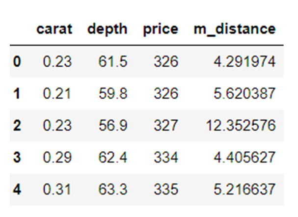
df_g= df[['carat', 'depth', 'price']].head(50)
df_g['m_distance'] = distance(x=df_g, data=df[['carat', 'depth', 'price']])
df_g.head()
B. Tukey’s method for outlier detection
Tukey method is also often called Box and Whisker or Box plot method.
Tukey method utilizes the Upper and lower range.
Upper range = 75th Percentile -k*IQR
Lower range = 25th Percentile + k* IQR
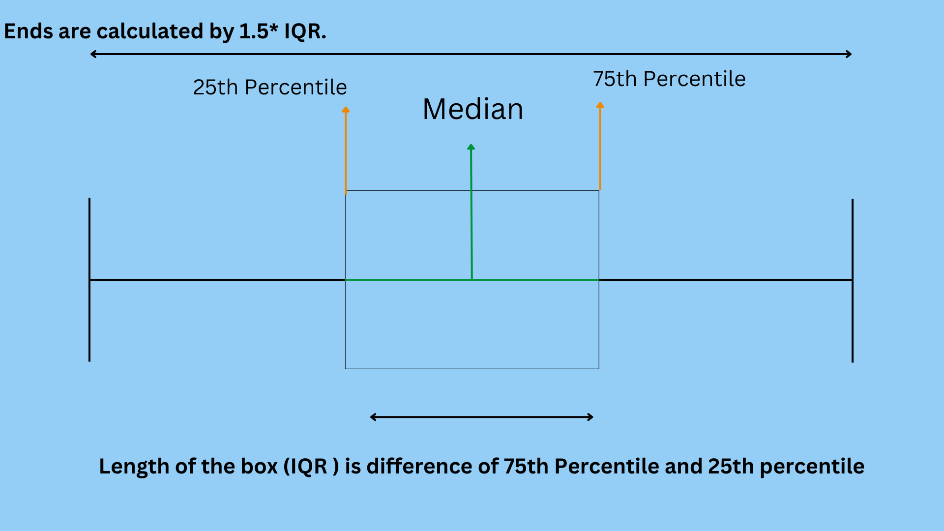
Let us see our Titanic data with age variable using a box plot.
sns.boxplot(titanic['age'].values)
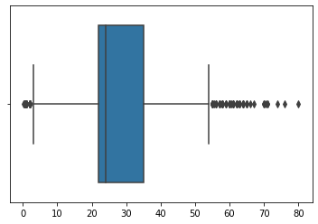
We can see in the image the box blot created by Seaborn shows many dots between the age of 55 and 80 are outliers not within the quartiles. We will detect lower and upper range by making a function outliers_detect.
def outliers_detect(x, k = 1.5):
    x = np.array(x).copy().astype(float)
    first = np.quantile(x, .25)
    third = np.quantile(x, .75)
    # IQR calculation
    iqr = third - first
    #Upper range and lower range
    lower = first - (k * iqr)
    upper = third + (k * iqr)
    return lower, upper
outliers_detect(titanic['age'], k = 1.5)
(2.5, 54.5)
Detection by PyCaret
We will be using the same dataset for detection by PyCaret.
from pycaret.anomaly import *
setup_anomaly_data = setup(df)
Pycaret is an open-source machine learning which uses an unsupervised learning model to detect outliers. It has a get_data method for using the dataset in pycaret itself, set_up for preprocessing task before detection, usually takes data frame but also has many other features like ignore_features, etc.
Other methods create_model for using an algorithm. We will first use Isolation Forest.
ifor = create_model("iforest")
plot_model(ifor)
ifor_predictions = predict_model(ifor, data = df)
print(ifor_predictions)
ifor_anomaly = ifor_predictions[ifor_predictions["Anomaly"] == 1]
print(ifor_anomaly.head())
print(ifor_anomaly.shape)
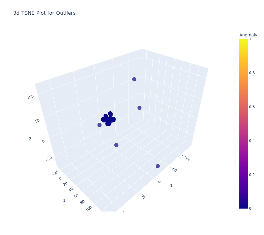
Anomaly 1 indicates outliers, and Anomaly 0 shows no outliers.
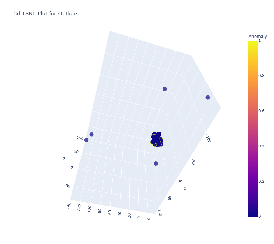
The yellow color here indicates outliers.
Now let us see another algorithm, K Nearest Neighbors (KNN)
knn = create_model("knn")
plot_model(knn)
knn_pred = predict_model(knn, data = df)
print(knn_pred)
knn_anomaly = knn_pred[knn_pred["Anomaly"] == 1]
knn_anomaly.head()
knn_anomaly.shape

Now we will use a clustering algorithm.
clus = create_model("cluster")
plot_model(clus)
clus_pred = predict_model(clus, data = df)
print(clus_pred)
clus_anomaly = clus_predictions[clus_pred["Anomaly"] == 1]
print(clus_anomaly.head())
clus_anomaly.shape
Anomaly Detection by PyOD
PyOD is a python library for the detection of outliers in multivariate data. It is good both for supervised and unsupervised learning.
from pyod.models.iforest import IForest
from pyod.models.knn import KNN
We imported the library and algorithm.
from pyod.utils.data import generate_data
from pyod.utils.data import evaluate_print
from pyod.utils.example import visualize
train= 300
test=100
contaminate = 0.1
X_train, X_test, y_train, y_test = generate_data(n_train=train, n_test=test, n_features=2,contamination=contaminate,random_state=42)
cname_alg = 'KNN' # the name of the algorithm is K Nearest Neighbors
c = KNN()
c.fit(X_train) #Fit the algorithm
y_trainpred = c.labels_
y_trainscores = c.decision_scores_
y_testpred = c.predict(X_test)
y_testscores = c.decision_function(X_test)
print("Training Data:")
evaluate_print(cname_alg, y_train, y_train_scores)
print("Test Data:")
evaluate_print(cname_alg, y_test, y_test_scores)
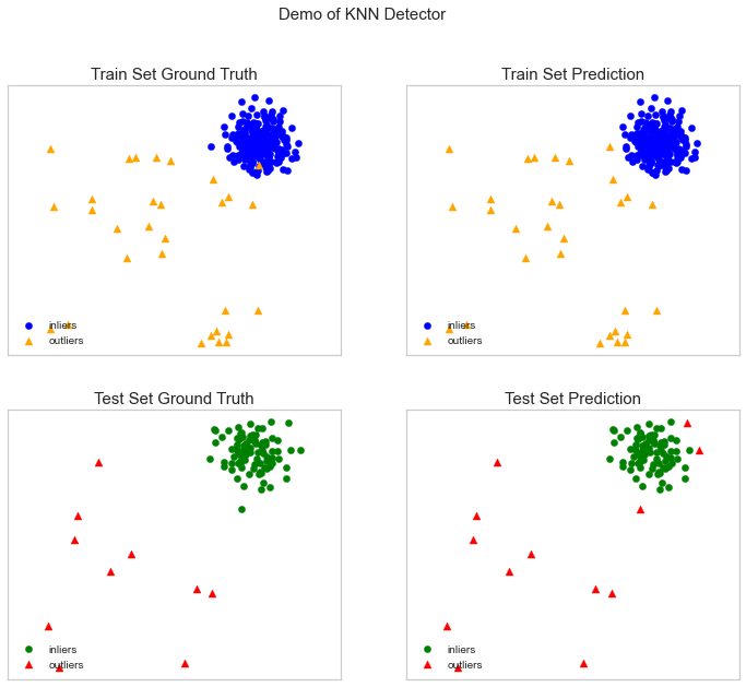
visualize(cname_alg, X_train, y_train, X_test, y_test, y_trainpred,y_testpred, show_figure=True, save_figure=True)
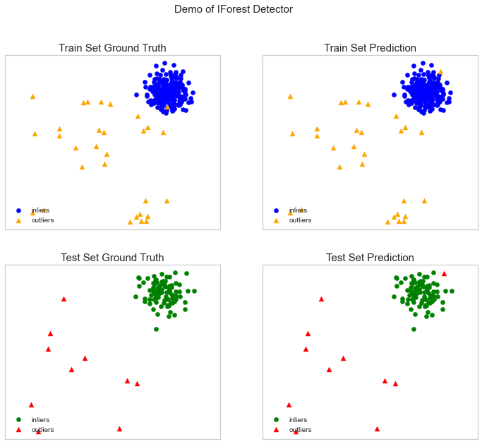
We will use the IForest algorithm.
fname_alg = 'IForest' # the name of the algorithm is K Nearest Neighbors
f = IForest()
f.fit(X_train) #Fit the algorithm
y_train_pred = c.labels_
y_train_scores = c.decision_scores_
y_test_pred = c.predict(X_test)
y_test_scores = c.decision_function(X_test)
print("Training Data:")
evaluate_print(fname_alg, y_train_pred, y_train_scores)
print("Test Data:")
evaluate_print(fname_alg, y_test_pred, y_test_scores)
visualize(fname_alg, X_train, y_train, X_test, y_test_pred, y_train_pred,y_test_pred, show_figure=True, save_figure=True)
Anomaly Detection by Prophet
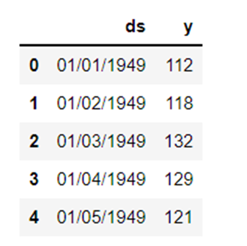
We will use the air passenger dataset with time series prophet/example_air_passengers.csv at main · aster28/prophet (github.com)
import prophet
from prophet import forecaster
from prophet import Prophet
m = Prophet()
data = pd.read_csv('air_pass.csv')
data.head()
data.columns = ['ds', 'y']
data['y'] = np.where(data['y'] != 0, np.log(data['y']), 0)
The Log of the y column enables no negative value. We split our data into train, test, and stored the prediction in the variable forecast.
train, test= train_test_split(data, random_state =42)
m.fit(train[['ds','y']])
forecast = m.predict(test)
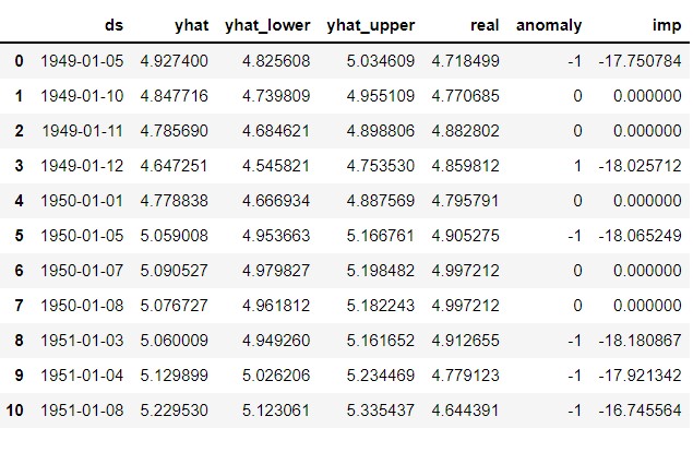
def detect(forecast):
    forcast = forecast[['ds', 'yhat', 'yhat_lower', 'yhat_upper']].copy()
    forcast['real']= data['y']
    forcast['anomaly'] =0
    forcast.loc[forcast['real']> forcast['yhat_upper'], 'anomaly']=1
    forcast.loc[forcast['real']< forcast['yhat_lower'], 'anomaly']=-1
    forcast['imp']=0
    in_range = forcast['yhat_upper']-forcast['yhat_lower']
    forcast.loc[forcast['anomaly']==1, 'imp'] = forcast['real']-forcast['yhat_upper']/in_range
    forcast.loc[forcast['anomaly']==-1, 'imp']=  forcast['yhat_lower']-forcast['real']/in_range
    return forcast
detect(forecast)
We took the anomaly as -1.
Conclusion
The process of finding outliers in a given dataset is called anomaly detection. Outliers are data objects that stand out from the rest of the object values in the dataset and don’t behave normally.
Anomaly detection tasks can use distance-based and density-based clustering methods to identify outliers as a cluster.
We here discuss anomaly detection’s various methods and explain them using the code on three datasets of Titanic, Air passengers, and Caret to understand uni-variate and Multi-variate outliers.
Key Points
1. Outliers or anomaly detection can be detected using the Box-Whisker method or by DBSCAN.
2. Euclidean distance method is used with the items not correlated.
3. Mahalanobis method is used with Multivariate outliers.
4. All the values or points are not outliers. Some are noises that ought to be garbage. Outliers are valid data that need to be adjusted.
5. We used PyCaret for outliers detection by using different algorithms where the anomaly is one, shown in yellow colors, and no outliers where the outlier is 0.
6. We used PyOD, which is the Python Outlier detection library. It has more than 40 algorithms. Supervised and unsupervised techniques it is used.
7. We used Prophet and defined the function detect to outline the outliers.
The media shown in this article is not owned by Analytics Vidhya and is used at the Author’s discretion.


