This article was published as a part of the Data Science Blogathon.
Introduction
The variance is the difference between the model and the ground truth value, whereas the error is the outcome of sensitivity to tiny perturbations in the training set. Excessive bias might cause an algorithm to miss unique relationships between the intended outputs and the features (underfitting). There is a high variance in the algorithm that models random noise in the training data (overfitting).
The bias-variance tradeoff is a characteristic of a model that states to lower the bias in estimated parameters, the variance of the parameter estimated across samples has increased. Mixture models and ensemble learning are one technique to resolve the bias-variance tradeoff. Voting, stacking, bagging, and boosting are the most used ensemble procedures.
This post goes through the four ensemble methods, with a quick brief of each and its pros and cons its python implementation.

Voting
A voting ensemble technique is a machine learning model that integrates predictions from various models to get a single final prediction. Because this ensemble method uses all of the training data to train the models, the models should be diverse.
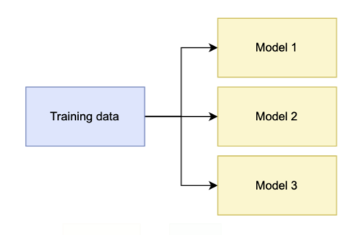
The simple goal of voting is to improve generalisation by accounting for each model’s faults separately, especially when the models are good at predictive modelling.
This method is effective for stochastic machine learning algorithms, such as neural networks, that produce a different model for each run. It’s also handy for integrating numerous fits of the same machine learning algorithm if the model predicts well when different hyperparameters had used.
Stacking
The stacking models had built up of base models (models fitted to the training data) and a meta-model (model that learns how to combine the predictions of the base models). A linear regression model is commonly used for regression tasks, whereas a logistic regression model had used for classification tasks.
The meta-model had trained using out-of-sample data predictions given by base models. In other words, data that had not been used for training the base models had passed as input, predictions made using these base models, and fit the meta-model using predicted values and ground truth labels.
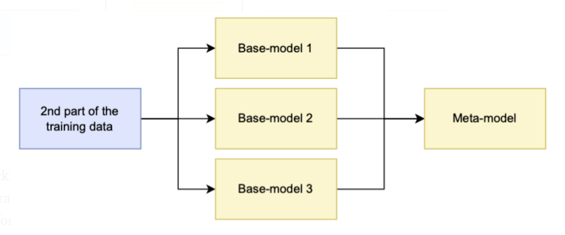
The meta-model input had determined by the task. The anticipated value is the input for regression tasks. The predicted value for the positive class is usually the input for binary classification tasks. The set of projected values for all classes had used for multiclass classification.
Blending is a type of stacking model often utilised in the literature. Blending models are trained on predictions made on a holdout dataset, whereas stacking models had trained on out-of-fold predictions produced during k-fold cross-validation.
It had developed to improve modelling performance, although it is not insured to result in a gain in all cases. If any base models serve like the stacking ensemble method, it should be preferable to use as it is more comfortable to define and maintain.
Bagging
Bagging is the practice of subsampling training data to improve a single type of classifier’s generalisation performance. This method works well with models that tend to overfit the data.
Bootstrapping (the name bagging originates from bootstrap + aggregating) is a process used to sub-sample the data. This method involves performing random sampling with replacement over the data, which means sections of the training data will overlap because the data is not separated but resampled.
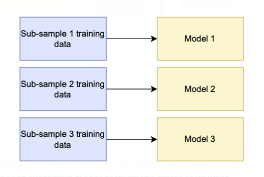
The final prediction for each data had obtained by regression voting, where predictions are the average of contributing models, or classification voting, where predictions are the majority vote of contributing models.
When using this method, keep in mind that the classifier’s hyperparameters do not change from subsample to subsample, and here improvement is usually not very significant. It is expensive because it can increase computational costs by 5 or 10 times, and this is a bias-reduction technique, so it won’t help you if you’re working with variance.
It is particularly effective when the data is overfitted, but not in case it is underfitting, because it minimises variance by better generalising.
Boosting
Boosting is an ensemble strategy for building models that use a sequence of weak learners to create the model. The basic principle is that each new model corrects the mistakes of the previous one.
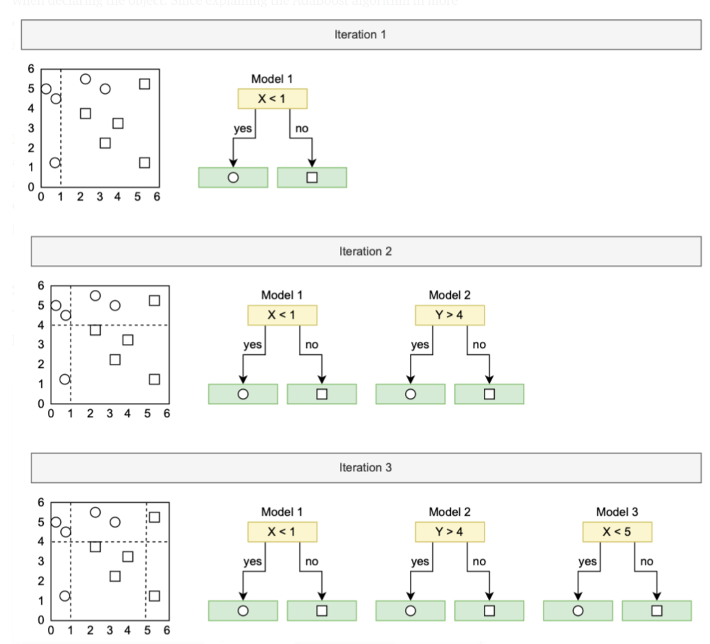
Even though there are several forms of boosting algorithms, such as Gradient Boosting or XGBoosting, AdaBoost was the first boosting method created for binary classification. Figure 9 shows how AdaBoosting works in a simple form to classify the circles and squares based on x and y attributes. The first model uses a vertical divider line to classify the data points. However, as can be seen, it incorrectly labels some of the data points in the circles.
As a result, the second model focuses on classifying these incorrectly categorised data points by raising their weight. This method had repeated for the number of estimators specified at the point item declared.
Boosting has been proved in the literature to produce accurate results since it is a resilient strategy that quickly prevents overfitting. It is, however, sensitive to outliers because each classifier is required to correct the errors in the predecessors, and it is also difficult to scale up because each estimator bases its correctness on the previous predictors.
Implementation
Now, we explore each of the ensemble methods.
import numpy as np
import matplotlib.pyplot as plt
import time

from sklearn.datasets import make_moons
from sklearn.ensemble._bagging import BaggingClassifier
from sklearn.ensemble import VotingClassifier, StackingClassifier, RandomForestClassifier, AdaBoostClassifier
from sklearn.svm import SVC
from sklearn.tree import DecisionTreeClassifier
from sklearn.linear_model import LogisticRegression
from sklearn.base import BaseEstimator

import torch
import torch.nn as nn
import torch.nn.functional as F

%matplotlib inline
We use the make_moons function to generate a random dataset that creates a circular shape.
np.random.seed(16)
tr_x, tr_y = make_moons(100, noise=0.3)
ts_x, ts_y = make_moons(1000, noise=0.3)
xx, yy = np.meshgrid(np.arange(-2, 3, 0.05), np.arange(-1.5, 2.0, 0.05))
zz = np.concatenate([xx.ravel()[:, np.newaxis], yy.ravel()[:, np.newaxis]], axis=1)
fig, axs = plt.subplots(1, 2, figsize=(10, 5))
axs[0].scatter(tr_x[:,0], tr_x[:,1], c=tr_y, cmap=plt.cm.Spectral)
axs[0].set_title('Train set')
axs[1].scatter(ts_x[:,0], ts_x[:,1], c=ts_y, cmap=plt.cm.Spectral)
axs[1].set_title('Test set')
plt.show()
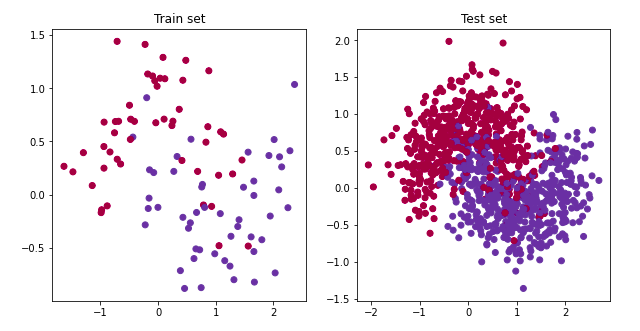
We used an SVM classifier, a decision tree classifier, and a logistic regression as benchmarks to evaluate the results of each ensemble method. The SVM classifier is a machine learning algorithm that finds a hyperplane in N-dimensional space (where N is the number of features), differentiating among data classes. The decision tree is a tree-structured classification in which internal nodes represent dataset features, branches represent decision rules, and each leaf node represents the outcome. The logistic regressor is a statistical analysis method that uses prior observations to predict a binary outcome.
- SVC: 84.2% accuracy and 0.07 sec runtime.
- Decision tree: 86.6% accuracy and 0.02 sec runtime.
- Logistic regression: 83.5% accuracy and 0.02 sec runtime.
clf_svc = SVC(C=10000, gamma='scale', probability=True)  # Support vector classifier
clf_dt = DecisionTreeClassifier()                        # Decision tree
clf_lr = LogisticRegression()                            # Logistic regressor
We use the below code to visualise the results of classification models.
time_now = time.time()
clf.fit(tr_x, tr_y)
p = clf.predict_proba(zz)
p = p.reshape((xx.shape[0], xx.shape[1], 2))
cax = axs[0].contourf(xx, yy, p[:,:,1], alpha=0.5, cmap=plt.cm.Spectral)
cbar = plt.colorbar(cax, ticks=[-1, 0, 1], ax=axs[0])
axs[0].scatter(tr_x[:,0], tr_x[:,1], c=tr_y,cmap=plt.cm.Spectral)
axs[0].set_title(f'Accuracy: {clf.score(ts_x, ts_y)}, time: {(time.time() - time_now):.2f} sec')
Voting
Below are the voting ensemble results with hard and soft voting
- Hard voting: 88.2% accuracy and 0.12 sec runtime.
- Decision tree: 87.3% accuracy and 0.09 sec runtime.
clf_hv = VotingClassifier(estimators=[('lr', clf_svc), ('rf', clf_dt), ('gnb', clf_lr)], voting='hard')
clf_sv = VotingClassifier(estimators=[('lr', clf_svc), ('rf', clf_dt), ('gnb', clf_lr)], voting='soft')
Both outputs resemble the decision tree plot in Figure 11. The models generalise better for the training set because they misclassify the red data points contained within the blue data points and vice versa. The main difference between hard and soft voting is visible in the image’s centre and where the region considered to be one class or the other had influenced by the weight assigned to the decision tree classifier.
One should replace clf.predict_proba(zz) by clf.predict(zz) since hard voting does not return probabilities.
time_now = time.time()
clf.fit(tr_x, tr_y)
p = clf.predict(zz)
p = p.reshape((xx.shape[0], xx.shape[1]))
cax = axs[axs_no].contourf(xx, yy, p[:,:], alpha=0.5, cmap=plt.cm.Spectral)
cbar = plt.colorbar(cax, ticks=[-1, 0, 1], ax=axs[axs_no])
axs[axs_no].scatter(tr_x[:,0], tr_x[:,1], c=tr_y,cmap=plt.cm.Spectral)
axs[axs_no].set_title(f'Hard voting (accuracy: {clf.score(ts_x, ts_y)}, time: {(time.time() - time_now):.2f} sec)', fontsize=15)
Stacking
The logistic regression is the meta-model for the stacking ensemble method. Since we are in a binary classification task, we used a 5-fold cross-validation for training.
- Stacking: 88.4% accuracy and 0.24 runtime.
clf = StackingClassifier(estimators=[('lr', clf_svc), ('rf', clf_dt), ('gnb', clf_lr)],
                         final_estimator=LogisticRegression(),
                         cv=5)
This model outperforms voting with the increase in execution time.
Bagging
- SVC: 87.7% accuracy and 0.19 sec runtime.
- Decision tree: 89.3% accuracy and 0.16 sec runtime.
- Logistic regression: 84.1% accuracy and 0.32 sec runtime.
clf_svc_bagging = BaggingClassifier(SVC(C=100000, gamma='scale', probability=True), n_estimators=100, max_samples=1.0)
clf_dt_bagging = BaggingClassifier(DecisionTreeClassifier(), n_estimators=100, max_samples=1.0)
clf_lr_bagging = BaggingClassifier(LogisticRegression(C=10000, solver='lbfgs'), n_estimators=100, max_samples=1.0)
The bagging approach for logistic regression creates a little non-linear model by merging many linear models. Outperform their respective models when compared to the benchmarks because they improve accuracy. It helps to reduce overfitting by voting over numerous trees with various training sets, which results in a considerable improvement for the decision tree.
The difference between Bagging and Random Forest is an intriguing topic to bring up here, as both systems appear to be pretty similar. As indicated in [2, 3], the number of features, as only a subset of elements had been chosen for the random forest, is the main difference.
clf_1 = RandomForestClassifier()
clf_2 = BaggingClassifier(DecisionTreeClassifier(), n_estimators=100, max_samples=1.0)
plot_results(clf_1, clf_2)
Boosting
Boosting Models performance below:
- SVC: 88.4% accuracy and 2.40 sec runtime.
- Decision tree: 87.2% accuracy and 0.02 sec runtime.
- Logistic regression: 83.7% accuracy and 0.15 sec runtime.
We observe the significant impact on the model’s performance based on two primary parameters. The learning rate, for starters, determines how quickly the weights/coefficients change. The number of estimators is similar to the number of trees in the model, and more trees are required to train our model as the learning rate decreases. In addition, the slower the learning rate is, the more resilient and efficient the model becomes. The learning rate and the number of estimators had set to 0.1 and 50.
clf_svc_boosting = AdaBoostClassifier(SVC(C=100000, gamma='scale', probability=True), n_estimators=50, learning_rate = 0.1)
clf_dt_boosting = AdaBoostClassifier(DecisionTreeClassifier(), n_estimators=50, learning_rate = 0.1)
clf_lr_boosting = AdaBoostClassifier(LogisticRegression(C=10000, solver='lbfgs'), n_estimators=50, learning_rate = 0.1)
While the SVM classifier’s results improved, the decision tree’s results did not, as it was still overfitting the training data.
clf_dt_1 = DecisionTreeClassifier(max_depth=1)
clf_dt_2 = DecisionTreeClassifier(max_depth=2)
clf_dt_3 = DecisionTreeClassifier()
Conclusion
We had familiarised ourselves with the four popular ensemble methods with their implementation.
Bagging helps to minimise prediction variance by generating additional data for training from a dataset by mixing repeats and combinations to form multi-sets of the original data. It is an iterative method for altering the weight of an observation based on its initial categorisation.
Boosting aims to raise the weight of observation if it was incorrectly classified, and it generally produces good predictive models. Ensemble modelling can significantly increase the model performance and perhaps make a difference in Leaderboard.
One can finalise the method based on the accuracy and computational cost. Every ensemble model has pros and cons, and choosing the best model is dependent on the problem and dataset that a person is working on.
I hope you found this article insightful.
The media shown in this article is not owned by Analytics Vidhya and is used at the Author’s discretion.


