


Introduction
Out of all the machine learning algorithms I have come across, the KNN algorithm has easily been the simplest to pick up. Despite its simplicity, it has proven to be incredibly effective at certain tasks (as you will see in this article).
What’s even better? It can be used for both classification and regression problems! KNN algorithm is by far more popularly used for classification problems, however. I have seldom seen KNN being implemented on any regression task. My aim here is to illustrate and emphasize how KNN can be equally effective when the target variable is continuous in nature.
Learning Objectives
- Understand the intuition behind KNN algorithms.
- Learn different ways to calculate distances between points.
- Practice implementing the algorithm in Python on the Big Mart Sales dataset.
If you want to understand the KNN algorithm in a course format, here is the link to our free course- K-Nearest Neighbors (KNN) Algorithm in Python and R
Table of contents
Understanding the Intuition Behind the KNN Algorithm
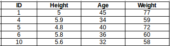
Let us start with a simple example. Consider the following table – it consists of the height, age, and weight (target) values for 10 people. As you can see, the weight value of ID11 is missing. We need to predict the weight of this person based on their height and age.
Note: The data in this table does not represent actual values. It is merely used as an example to explain this concept.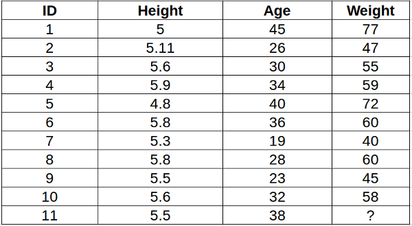
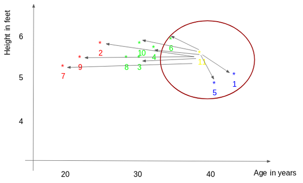
For a clearer understanding of this, below is the plot of height versus age from the above table:
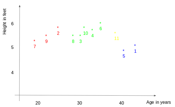
In the above graph, the y-axis represents the height of a person (in feet) and the x-axis represents the age (in years). The points are numbered according to the ID values. The yellow point (ID 11) is our test point.
If I ask you to identify the weight of ID11 based on the plot, what would be your answer? You would likely say that since ID11 is closer to points 5 and 1, so it must have a weight similar to these IDs, probably between 72-77 kgs (weights of ID1 and ID5 from the table). That actually makes sense, but how do you think the algorithm predicts the values? We will find that out in this article.
Here is a free video-based course to help you understand the KNN algorithm – K-Nearest Neighbors (KNN) Algorithm in Python and R
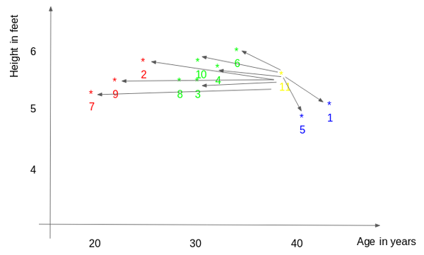
How Does the KNN Algorithm Work?
As we saw above, the KNN algorithm can be used for both classification and regression problems. The KNN algorithm uses ‘feature similarity’ to predict the values of any new data points. This means that the new point is assigned a value based on how closely it resembles the points in the training set. From our example, we know that ID11 has height and age similar to ID1 and ID5, so the weight would also approximately be the same.
Had it been a classification problem, we would have taken the mode as the final prediction. In this case, we have two values of weight – 72 and 77. Any guesses on how the final value will be calculated? The average of the values is taken to be the final prediction.
Below is a stepwise explanation of the algorithm:
1. First, the distance between the new point and each training point is calculated.
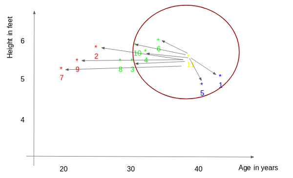
2. The closest k data points are selected (based on the distance). In this example, points 1, 5, and 6 will be selected if the value of k is 3. We will further explore the method to select the right value of k later in this article.

3. The average of these data points is the final prediction for the new point. Here, we have the weight of ID11 = (77+72+60)/3 = 69.66 kg.
In the next few sections, we will discuss each of these three steps in detail.
How to Calculate the Distance Between Points?
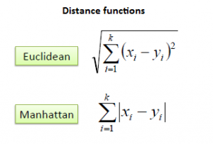
The first step is to calculate the distance between the new point and each training point. There are various methods for calculating this distance, of which the most commonly known methods are – Euclidian, Manhattan (for continuous), and Hamming distance (for categorical).
- Euclidean Distance: Euclidean distance is calculated as the square root of the sum of the squared differences between a new point (x) and an existing point (y).
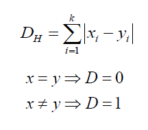
- Manhattan Distance: This is the distance between real vectors using the sum of their absolute difference.

- Hamming Distance: It is used for categorical variables. If the value (x) and the value (y) are the same, the distance D will be equal to 0. Otherwise D=1.
There is also Minkowski distance which is a generalized form of Euclidean and manhattan distances.
Once the distance of a new observation from the points in our training set has been measured, the next step is to pick the closest points. The number of points to be considered is defined by the value of k.
How to Choose the K-factor?
The second step is to select the k value. This determines the number of neighbors we look at when we assign a value to any new observation.
In our example, for a value k = 3, the closest points are ID1, ID5, and ID6.
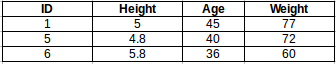
The prediction of weight for ID11 will be:
ID11 = (77+72+60)/3

ID11 = 69.66 kg
For the value of k=5, the closest point will be ID1, ID4, ID5, ID6, and ID10.
The prediction for ID11 will be:
ID 11 =  (77+59+72+60+58)/5

ID 11 = 65.2 kg
We notice that based on the k value, the final result tends to change. Then how can we figure out the optimum value of k? Let us decide based on the error calculation for our train and validation set (after all, minimizing the error is our final goal!).
Have a look at the below graphs for training error and validation error for different values of k.
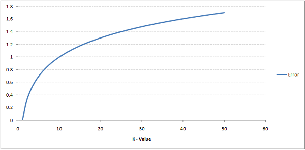
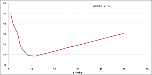
For a very low value of k (suppose k=1), the model is overfitting the training data, which leads to a high error rate on the validation set. On the other hand, for a high value of k, the model performs poorly on both the train and validation sets. If you observe closely, the validation error curve reaches a minimum at a value of k = 9. This value of k is the optimum value of the model (it will vary for different datasets). This curve is known as an ‘elbow curve‘ (because it has a shape like an elbow) and is usually used to determine the k value.
You can also use the grid search technique to find the best k value. We will implement this in the next section.
Implementation of KNN Algorithm Using Python
By now, you must have a clear understanding of the algorithm. If you have any questions regarding the same, please use the comments section below, and I will be happy to answer them. We will now go ahead and implement the algorithm on a dataset. I have used the Big Mart sales dataset to show the implementation; you can download it from this link.
The full Python code is below, but we have a really cool coding window here where you can code your own k-Nearest Neighbor model in Python:
Step 1: Read the file
import pandas as pd
df = pd.read_csv('train.csv')
df.head()
Step 2: Impute missing values
df.isnull().sum()
#missing values in Item_weight and Outlet_size needs to be imputed
mean = df['Item_Weight'].mean() #imputing item_weight with mean
df['Item_Weight'].fillna(mean, inplace =True)

mode = df['Outlet_Size'].mode() #imputing outlet size with mode
df['Outlet_Size'].fillna(mode[0], inplace =True)
Step 3: Deal with categorical variables and drop the id columns
df.drop(['Item_Identifier', 'Outlet_Identifier'], axis=1, inplace=True)
df = pd.get_dummies(df)
Step 4: Create a train and a test set
from sklearn.model_selection import train_test_split
train , test = train_test_split(df, test_size = 0.3)

x_train = train.drop('Item_Outlet_Sales', axis=1)
y_train = train['Item_Outlet_Sales']

x_test = test.drop('Item_Outlet_Sales', axis = 1)
y_test = test['Item_Outlet_Sales']
Step 5: Preprocessing – Scaling the features
from sklearn.preprocessing import MinMaxScaler
scaler = MinMaxScaler(feature_range=(0, 1))

x_train_scaled = scaler.fit_transform(x_train)
x_train = pd.DataFrame(x_train_scaled)

x_test_scaled = scaler.fit_transform(x_test)
x_test = pd.DataFrame(x_test_scaled)
Step 6: Let us have a look at the error rate for different k values
#import required packages
from sklearn import neighbors
from sklearn.metrics import mean_squared_error
from math import sqrt
import matplotlib.pyplot as plt
%matplotlib inline
rmse_val = [] #to store rmse values for different k
for K in range(20):
    K = K+1
    model = neighbors.KNeighborsRegressor(n_neighbors = K)

    model.fit(x_train, y_train)  #fit the model
    pred=model.predict(x_test) #make prediction on test set
    error = sqrt(mean_squared_error(y_test,pred)) #calculate rmse
    rmse_val.append(error) #store rmse values
    print('RMSE value for k= ' , K , 'is:', error)
Output:
RMSE value for k = 1 is: 1579.8352322344945
RMSE value for k = 2 is: 1362.7748806138618
RMSE value for k = 3 is: 1278.868577489459
RMSE value for k = 4 is: 1249.338516122638
RMSE value for k = 5 is: 1235.4514224035129
RMSE value for k = 6 is: 1233.2711649472913
RMSE value for k = 7 is: 1219.0633086651026
RMSE value for k = 8 is: 1222.244674933665
RMSE value for k = 9 is: 1219.5895059285074
RMSE value for k = 10 is: 1225.106137547365
RMSE value for k = 11 is: 1229.540283771085
RMSE value for k = 12 is: 1239.1504407152086
RMSE value for k = 13 is: 1242.3726040709887
RMSE value for k = 14 is: 1251.505810196545
RMSE value for k = 15 is: 1253.190119191363
RMSE value for k = 16 is: 1258.802262564038
RMSE value for k = 17 is: 1260.884931441893
RMSE value for k = 18 is: 1265.5133661294733
RMSE value for k = 19 is: 1269.619416217394
RMSE value for k = 20 is: 1272.10881411344
#plotting the rmse values against k values
curve = pd.DataFrame(rmse_val) #elbow curve
curve.plot()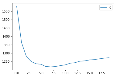
As we discussed, when we take k=1, we get a very high RMSE value. The RMSE value decreases as we increase the k value. At k= 7, the RMSE is approximately 1219.06 and shoots upon further increasing the k value. We can safely say that k=7 will give us the best result in this case.
These are the predictions using our training dataset. Let us now predict the values for test data and make a submission.
Step 7: Make predictions on the test dataset
#reading test and submission files
test = pd.read_csv('test.csv')
submission = pd.read_csv('SampleSubmission.csv')
submission['Item_Identifier'] = test['Item_Identifier']
submission['Outlet_Identifier'] = test['Outlet_Identifier']

#preprocessing test dataset
test.drop(['Item_Identifier', 'Outlet_Identifier'], axis=1, inplace=True)
test['Item_Weight'].fillna(mean, inplace =True)
test = pd.get_dummies(test)
test_scaled = scaler.fit_transform(test)
test = pd.DataFrame(test_scaled)

#predicting on the test set and creating submission file
predict = model.predict(test)
submission['Item_Outlet_Sales'] = predict
submission.to_csv('submit_file.csv',index=False)
On submitting this file, I get an RMSE of 1279.5159651297.
Step 8: Implementing GridsearchCV
For deciding the value of k, plotting the elbow curve every time is a cumbersome and tedious process. You can simply use grid search to find the best parameter value.
from sklearn.model_selection import GridSearchCV
params = {'n_neighbors':[2,3,4,5,6,7,8,9]}

knn = neighbors.KNeighborsRegressor()

model = GridSearchCV(knn, params, cv=5)
model.fit(x_train,y_train)
model.best_params_
Output:
{'n_neighbors': 7}Conclusion
In this article, we covered the workings of the KNN algorithm and its implementation in Python. It’s one of the most basic yet effective machine-learning models. For KNN implementation in R, you can go through this tutorial: kNN Algorithm using R. You can also go for our free course – K-Nearest Neighbors (KNN) Algorithm in Python and R, to further your foundations of KNN.
In this article, we used the KNN model directly from the scikit-learn library. You can also implement KNN from scratch (I recommend this!), which is covered in this article: KNN simplified.
If you think you know KNN well and have a solid grasp of the technique, test your skills in this MCQ quiz: 30 questions on kNN Algorithm. Good luck!
Key Takeaways
- We have learned how to implement KNN in Python.
- We have learned to compute the optimum value of the K hyper-parameter.
- We have learned that the KNN regression model is useful in many regression problems.
Frequently Asked Questions
A. K nearest neighbors is a supervised machine learning algorithm that can be used for classification and regression tasks. In this, we calculate the distance between features of test data points against those of train data points. Then, we take a mode or mean to compute prediction values.
A. Yes, we can use KNN for regression. Here, we take the k nearest values of the target variable and compute the mean of those values. Those k nearest values act like regressors of linear regression.
A. We can use the elbow method where we plot the test data set error vs. k-value for different k-values. We can choose K, where the improvement in error is negligible.
A. KNN (K-Nearest Neighbors) Classifier is a type of machine learning algorithm used for classification tasks. It is a non-parametric algorithm, which means it does not make any assumptions about the underlying distribution of the data.
In KNN Classifier, a new data point is classified based on its proximity to the K nearest neighbors in the training set. The proximity is measured using a distance metric, such as Euclidean distance or Manhattan distance. The class of the majority of the K nearest neighbors is then assigned to the new data point as its predicted class.
An avid reader and blogger who loves exploring the endless world of data science and artificial intelligence. Fascinated by the limitless applications of ML and AI; eager to learn and discover the depths of data science.