This article was published as a part of the Data Science Blogathon
Why Julia is future of Data Science and learns how to write your first code

Introduction
Julia is a high-level and general-purpose language that can be used to write code that is fast to execute and easy to implement for scientific calculations. The language is designed to keep all the needs of scientific researchers and data scientists to optimize the experimentation and design implementation. Julia (programming language).
Python is still famous among data science enthusiasts as they get an ecosystem with loaded libraries to makes the work of data science and analysis faster and more convenient.
“Julia was built for scientific computing, machine learning, data mining, large-scale linear algebra, distributed and parallel computing”—developers behind the Julia language.
Python isn’t fast or convenient enough and it comes with securities variabilities as most of the libraries are built from other languages such a JavaScript, Java, C, and C++. The fast execution and convenient development make it quite attractive among the data science community and the majority of libraries are directly written in Julia to provide an extra layer of security. InfoWorld.
According to Jeremy Howard “Python is not the future of machine learning”.
In his recent video, he talks about how Python is frustrating when it comes to running machine learning models as you have to use other languages libraries such as CUDA and to run parallel computing you must use other libraries which makes it quite difficult. He also suggests how Julia is going to be the future of machine learning and if you want to become future-proof and have free time to learn a new language I will suggest you start with Julia.
Overview
In this article, I will be discussing the advantages of Julia’s language and I will display how it’s easy to use just like pandas and seaborn in python. I will use simple examples and a few lines of code to demonstrate data manipulation and data visualization. In this article, I will be using the famous Heart Disease UCI | Kaggle Dataset which has a binary classification of Heart Disease based on multiple factors. The dataset is small and clean so it’s the best example we can use to see how simple Julia has become.
Julia
While comparing with Python, Julia takes lead in multiple fields as mentioned below.
Julia is fast
Python can be made optimized by using external libraries and optimization tools, but Julia is faster by default as it comes with JIT compilation and type declarations.
Math-friendly syntax
Julia attracts non-programmer scientists by providing simple syntax for math operations which are similar to the non-computing world.
Automatic memory management
Julia is better than Python in terms of memory allocation, and it provides you more freedom to manually control garbage collection. Whereas in python you are constantly freeing memory and collecting information about memory usage which can be daunting in some cases.
Superior parallelism
It’s necessary to use all available resources while running scientific algorithms such as running it on parallels computing with a multi-core processor. For Python, you need to use external packages for parallel computing or serialized and deserialized operations between threads which can be hard to use. For Julia, it’s much simpler in implementation as it inherently comes with parallelism.
Native machine learning libraries
Flux is a machine learning library for Julia and there are other deep learning frameworks under development that are entirely written in Julia and can be modified as needed by the user. These libraries come with GPU acceleration, so you don’t need to worry about the slow training of deep learning models.
For more information, you can read the InfoWorld article.
Exploring Heart Disease Dataset
Before you follow my code, I want to look into A tutorial on DataFrames.jl prepared for JuliaCon2021 as most of my code is inspired by the live conference.
Before you start coding you need to set up your Julia repl, either use JuliaPro or set up your VS code for Julia and if you are using a cloud notebook just like me, I will suggest you add the below code into your docker file and build it. Docker code below only works for Deepnote only.
The output of the code shows a limited number of columns for the compact view but in reality, it has 14 columns.
FROM gcr.io/deepnote-200602/templates/deepnote
RUN wget https://julialang-s3.julialang.org/bin/linux/x64/1.6/julia-1.6.2-linux-x86_64.tar.gz &&
    tar -xvzf julia-1.6.2-linux-x86_64.tar.gz &&
    sudo mv julia-1.6.2 /usr/lib/ &&
    sudo ln -s /usr/lib/julia-1.6.2/bin/julia /usr/bin/julia &&
    rm julia-1.6.2-linux-x86_64.tar.gz &&
    julia  -e "using Pkg;pkg"add IJulia LinearAlgebra SparseArrays Images MAT""
ENV DEFAULT_KERNEL_NAME "julia-1.6.2"
Installing Julia packages
The method below will help you download and install all multiple libraries at once.
import Pkg; Pkg.add(["CSV","CategoricalArrays",
"Chain", "DataFrames", "GLM", "Plots", "Random", "StatsPlots",
"Statistics","Interact", "Blink"])
Importing Packages
We will be focusing more on loading CVS files, data manipulation, and visualization.
using CSV
using CategoricalArrays
using Chain
using DataFrames
using GLM
using Plots
using Random
using StatsPlots
using Statistics

ENV["LINES"] = 20 # to limit number of rows.
ENV["COLUMNS"] = 20 # to limit number of columns
Loading Data
We are using the famous Heart Disease UCI | Kaggle dataset for our beginner-level code for data analysis. We will be focusing on the coding part.
Features:
- age
- sex
- chest pain type (4 values)
- resting blood pressure
- serum cholesterol in mg/dl
- fasting blood sugar > 120 mg/dl
- resting electrocardiographic results (values 0,1,2)
- maximum heart rate achieved
- exercise-induced angina
- oldpeak
- the slope of the peak exercise ST segment
- number of major vessels
- thal: 3 to 7 where 5 is normal.
Simply Use `CSV.read()` just like pandas `pd.read_csv()` and your data will be loaded as data frame.
df_raw = CSV.read("/work/Data/Heart Disease Dataset.csv", DataFrame)
303 rows × 14 columns
| age | sex | cp | trestbps | chol | fbs | restecg | thalach | exang | oldpeak | slope | ca | thal | target | |
|---|---|---|---|---|---|---|---|---|---|---|---|---|---|---|
| Int64 | Int64 | Int64 | Int64 | Int64 | Int64 | Int64 | Int64 | Int64 | Float64 | Int64 | Int64 | Int64 | Int64 | |
| 1 | 63 | 1 | 3 | 145 | 233 | 1 | 0 | 150 | 0 | 2.3 | 0 | 0 | 1 | 1 |
| 2 | 37 | 1 | 2 | 130 | 250 | 0 | 1 | 187 | 0 | 3.5 | 0 | 0 | 2 | 1 |
| 3 | 41 | 0 | 1 | 130 | 204 | 0 | 0 | 172 | 0 | 1.4 | 2 | 0 | 2 | 1 |
| 4 | 56 | 1 | 1 | 120 | 236 | 0 | 1 | 178 | 0 | 0.8 | 2 | 0 | 2 | 1 |
| 5 | 57 | 0 | 0 | 120 | 354 | 0 | 1 | 163 | 1 | 0.6 | 2 | 0 | 2 | 1 |
| Operation | pandas | DataFrames.jl |
|---|---|---|
| Cell indexing by location | df.iloc[1, 1] |
df[2, 2] |
| Row slicing by location | df.iloc[1:3] |
df[2:3, :] |
| Column slicing by location | df.iloc[:, 1:] |
df[:, 2:end] |
| Row indexing by label | df.loc['c'] |
df[findfirst(==('c'), df.id), :] |
| Column indexing by label | df.loc[:, 'x'] |
df[:, :x] |
| Column slicing by label | df.loc[:, ['x', 'z']] |
df[:, [:x, :z]] |
df.loc[:, 'x':'z'] |
df[:, Between(:x, :z)] |
|
| Mixed indexing | df.loc['c'][1] |
df[findfirst(==('c'), df.id), 2] |
For more Information on Comparison with Python/R/Stata · DataFrames.jl (juliadata.org)
Checking the shape of the Dataframe
size(df_raw)
output
(303, 14)
Checking Multiple features distributions. We can observe mean, min, max, and missing all in one, using `describe()`
describe(df_raw)
| variable | mean | min | median | max | nmissing | eltype | |
|---|---|---|---|---|---|---|---|
| Symbol | Float64 | Real | Float64 | Real | Int64 | DataType | |
| 1 | age | 54.2013 | 34 | 55.0 | 77 | 0 | Int64 |
| 2 | sex | 0.660066 | 0 | 1.0 | 1 | 0 | Int64 |
| 3 | cp | 0.874587 | 0 | 1.0 | 3 | 0 | Int64 |
| 4 | trestbps | 131.007 | 94 | 130.0 | 200 | 0 | Int64 |
| 5 | chol | 251.627 | 141 | 248.0 | 564 | 0 | Int64 |
| 6 | fbs | 0.128713 | 0 | 0.0 | 1 | 0 | Int64 |
| 7 | restecg | 0.547855 | 0 | 1.0 | 2 | 0 | Int64 |
| 8 | thalach | 150.29 | 71 | 155.0 | 192 | 0 | Int64 |
| 9 | exang | 0.330033 | 0 | 0.0 | 1 | 0 | Int64 |
| 10 | oldpeak | 1.06337 | 0.0 | 0.8 | 5.6 | 0 | Float64 |
| 11 | slope | 1.40924 | 0 | 1.0 | 2 | 0 | Int64 |
| 12 | ca | 0.70297 | 0 | 0.0 | 4 | 0 | Int64 |
| 13 | thal | 2.30033 | 0 | 2.0 | 3 | 0 | Int64 |
| 14 | target | 0.547855 | 0 | 1.0 | 1 | 0 | Int64 |
Data select
we can convert columns into categorical types by using `:fbs => categorical => :fbs` and we have used between to select multiple columns at once. The select function is simple, for selecting columns and manipulating the types.
df = select(df_raw,:age,:sex => categorical => :sex,
            Between(:cp, :chol),
            :fbs => categorical => :fbs,:restecg,:thalach,
            :exang => categorical => :exang,
            Between(:oldpeak,:thal),
            :target => categorical => :target
            )
303 rows × 14 columns
| age | sex | cp | trestbps | chol | fbs | restecg | thalach | exang | oldpeak | slope | ca | thal | target | |
|---|---|---|---|---|---|---|---|---|---|---|---|---|---|---|
| Int64 | Cat… | Int64 | Int64 | Int64 | Cat… | Int64 | Int64 | Cat… | Float64 | Int64 | Int64 | Int64 | Cat… | |
| 1 | 47 | 1 | 2 | 108 | 243 | 0 | 1 | 152 | 0 | 0.0 | 2 | 0 | 2 | 0 |
| 2 | 35 | 1 | 0 | 126 | 282 | 0 | 0 | 156 | 1 | 0.0 | 2 | 0 | 3 | 0 |
| 3 | 68 | 1 | 0 | 144 | 193 | 1 | 1 | 141 | 0 | 3.4 | 1 | 2 | 3 | 0 |
| 4 | 50 | 0 | 0 | 110 | 254 | 0 | 0 | 159 | 0 | 0.0 | 2 | 0 | 2 | 1 |
| 5 | 49 | 0 | 1 | 134 | 271 | 0 | 1 | 162 | 0 | 0.0 | 1 | 0 | 2 | 1 |
| 6 | 40 | 1 | 0 | 110 | 167 | 0 | 0 | 114 | 1 | 2.0 | 1 | 0 | 3 | 0 |
| 7 | 45 | 1 | 0 | 142 | 309 | 0 | 0 | 147 | 1 | 0.0 | 1 | 3 | 3 | 0 |
| 8 | 57 | 0 | 0 | 120 | 354 | 0 | 1 | 163 | 1 | 0.6 | 2 | 0 | 2 | 1 |
| 9 | 62 | 0 | 0 | 140 | 394 | 0 | 0 | 157 | 0 | 1.2 | 1 | 0 | 2 | 1 |
| 10 | 34 | 1 | 3 | 118 | 182 | 0 | 0 | 174 | 0 | 0.0 | 2 | 0 | 2 | 1 |
Using Chain
if you want to apply multiple operations on your datasets all at once, I will suggest you use chain, in R it’s equivalent to `%>%`.
- the dropmissing will drop missing values from the database, we don’t have any missing, so this is simply for a showcase.
- the
groupbyfunction groups the data frame by the passed column - the
combinefunction that combines the rows of a data frame by some function
for more operations check out Chain.jl documentation
you can see the results of how I have grouped the data frame by target and then combine 5 columns to get the mean values.
@chain df_raw begin
    dropmissing
    groupby(:target)
    combine([:age, :sex, :chol, :restecg, :slope] .=> mean)
end
| target | age_mean | sex_mean | chol_mean | restecg_mean | slope_mean | |
|---|---|---|---|---|---|---|
| Int64 | Float64 | Float64 | Float64 | Float64 | Float64 | |
| 1 | 0 | 56.6277 | 0.824818 | 254.073 | 0.489051 | 1.14599 |
| 2 | 1 | 52.1988 | 0.524096 | 249.608 | 0.596386 | 1.62651 |
another simple way to use group by and combine is by using names(df, Real) which returns all the columns with real values, which mean not integers or categorical columns.
@chain df_raw begin
    groupby(:target)
    combine(names(df, Real) .=> mean)
end
| target | age_mean | cp_mean | trestbps_mean | chol_mean | restecg_mean | thalach_mean | oldpeak_mean | slope_mean | ca_mean | thal_mean | |
|---|---|---|---|---|---|---|---|---|---|---|---|
| Int64 | Float64 | Float64 | Float64 | Float64 | Float64 | Float64 | Float64 | Float64 | Float64 | Float64 | |
| 1 | 0 | 56.6277 | 0.518248 | 133.73 | 254.073 | 0.489051 | 138.65 | 1.68686 | 1.14599 | 1.16788 | 2.58394 |
| 2 | 1 | 52.1988 | 1.16867 | 128.759 | 249.608 | 0.596386 | 159.898 | 0.548795 | 1.62651 | 0.319277 | 2.06627 |
You can also add multiple columns using groupby and combine them by nrows which will display a number of rows for each sub-group.
@chain df_raw begin
    groupby([:target, :sex])
    combine(nrow)
end
| target | sex | nrow | |
|---|---|---|---|
| Int64 | Int64 | Int64 | |
| 1 | 0 | 0 | 24 |
| 2 | 0 | 1 | 113 |
| 3 | 1 | 0 | 79 |
| 4 | 1 | 1 | 87 |
You can also combine it and then unstack as shown below. So that one category becomes an index and another becomes a column.
@chain df_raw begin
    groupby([:target, :sex])
    combine(nrow)
    unstack(:target, :sex, :nrow)
end
| target | 0 | 1 | |
|---|---|---|---|
| Int64 | Int64? | Int64? | |
| 1 | 0 | 24 | 113 |
| 2 | 1 | 79 | 87 |
Groupby
The simple group by the function will show all groups at a time and access the specific group you need to hack it.
gd = groupby(df_raw, :target)
First Group (137 rows): target = 0
| age | sex | cp | trestbps | chol | fbs | restecg | thalach | exang | oldpeak | slope | ca | thal | target | |
|---|---|---|---|---|---|---|---|---|---|---|---|---|---|---|
| Int64 | Int64 | Int64 | Int64 | Int64 | Int64 | Int64 | Int64 | Int64 | Float64 | Int64 | Int64 | Int64 | Int64 | |
| 1 | 47 | 1 | 2 | 108 | 243 | 0 | 1 | 152 | 0 | 0.0 | 2 | 0 | 2 | 0 |
| 2 | 35 | 1 | 0 | 126 | 282 | 0 | 0 | 156 | 1 | 0.0 | 2 | 0 | 3 | 0 |
| 3 | 68 | 1 | 0 | 144 | 193 | 1 | 1 | 141 | 0 | 3.4 | 1 | 2 | 3 | 0 |
| 4 | 40 | 1 | 0 | 110 | 167 | 0 | 0 | 114 | 1 | 2.0 | 1 | 0 | 3 | 0 |
| 5 | 45 | 1 | 0 | 142 | 309 | 0 | 0 | 147 | 1 | 0.0 | 1 | 3 | 3 | 0 |
Last Group (166 rows): target = 1
| age | sex | cp | trestbps | chol | fbs | restecg | thalach | exang | oldpeak | slope | ca | thal | target | |
|---|---|---|---|---|---|---|---|---|---|---|---|---|---|---|
| Int64 | Int64 | Int64 | Int64 | Int64 | Int64 | Int64 | Int64 | Int64 | Float64 | Int64 | Int64 | Int64 | Int64 | |
| 1 | 50 | 0 | 0 | 110 | 254 | 0 | 0 | 159 | 0 | 0.0 | 2 | 0 | 2 | 1 |
| 2 | 49 | 0 | 1 | 134 | 271 | 0 | 1 | 162 | 0 | 0.0 | 1 | 0 | 2 | 1 |
| 3 | 57 | 0 | 0 | 120 | 354 | 0 | 1 | 163 | 1 | 0.6 | 2 | 0 | 2 | 1 |
| 4 | 62 | 0 | 0 | 140 | 394 | 0 | 0 | 157 | 0 | 1.2 | 1 | 0 | 2 | 1 |
we can use :
gd[(target=0,)] | gd[Dict(:target => 0)] | gd[(0,)]
to get a specific group that we are focusing on, this helps us a lot in the long run. gd[1] will be shown the first group which is target =0.
gd[1]
| age | sex | cp | trestbps | chol | fbs | restecg | thalach | exang | oldpeak | slope | ca | thal | target | |
|---|---|---|---|---|---|---|---|---|---|---|---|---|---|---|
| Int64 | Int64 | Int64 | Int64 | Int64 | Int64 | Int64 | Int64 | Int64 | Float64 | Int64 | Int64 | Int64 | Int64 | |
| 1 | 47 | 1 | 2 | 108 | 243 | 0 | 1 | 152 | 0 | 0.0 | 2 | 0 | 2 | 0 |
| 2 | 35 | 1 | 0 | 126 | 282 | 0 | 0 | 156 | 1 | 0.0 | 2 | 0 | 3 | 0 |
| 3 | 68 | 1 | 0 | 144 | 193 | 1 | 1 | 141 | 0 | 3.4 | 1 | 2 | 3 | 0 |
| 4 | 40 | 1 | 0 | 110 | 167 | 0 | 0 | 114 | 1 | 2.0 | 1 | 0 | 3 | 0 |
Density Plot
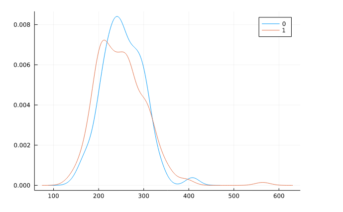
For this, we use a density plot from the StatsPlots.jl package. This package contains statistical recipes that extend the Plots.jl functionality. Just like seaborn with simple code, we can get our density plot with the separate groups are defined by colors.
We are going to group it by target columns and display cholesterol.
@df df density(:chol, group=:target)
Output:

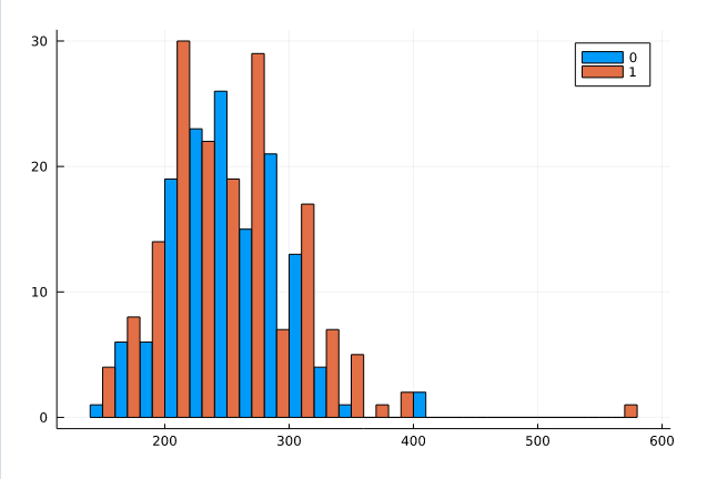
Group Histogram
Similar to density plot you can plot grouphist which is grouped by target and display cholesterols.
@df df_raw groupedhist(:chol, group = :target, bar_position = :dodge)

Multiple plots
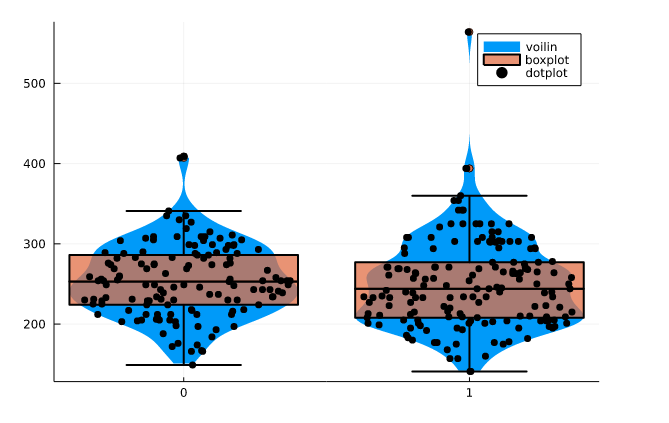
You can plot multiple graphs on the same figure by using! at the end of the function name for example `boxplot!()`. I have shown the example below of violin plot, boxplot, and dotplot on cholesterol which is grouped by the target.
@df df_raw violin(string.(:target), :chol, linewidth=0,label = "voilin")
@df df_raw boxplot!(string.(:target), :chol, fillalpha=0.75, linewidth=2,label = "boxplot")
@df df_raw dotplot!(string.(:target), :chol, marker=(:black, stroke(0)),label = "dotplot")

Predictive Model
I have used the glm model just like in R you can use y~x to train the model. The example below has x= trestbps, age, chol, thalach, oldpeak, slope, ca, and y= target which is binary. We are going to train our generalized linear model on binomial distribution to predict heart disease which is the target.
probit = glm(@formula(target ~ trestbps	 + age + chol + thalach + oldpeak + slope + ca),
             df_raw, Binomial(), ProbitLink())
Output:
Conclusion
In this article, we have showcased how simple the Julia language is and how powerful it is when it comes to scientific calculations. With few lines of code, we have discovered that this language has the potential to overtake python as it has similar syntax but higher performance. It’s still new to data science but I am sure tit the future of machine learning and Artificial intelligence.
To be honest I am also learning new stuff about Julia every day and if you want to know more about parallel computing and deep learning using GPU or Machine learning in general do look out for my other article in the future.
I haven’t done more exploration on the predictive models and data manipulation at this is an introductory article with generalized examples. So, if you think there is more, I could do, do let me know and I will try to add it in my next article.
Do follow me on LinkedIn where I post Articles on Data Science every week.
The media shown in this article are not owned by Analytics Vidhya and are used at the Author’s discretion.


