This article was published as a part of the Data Science Blogathon.
Introduction on Classification
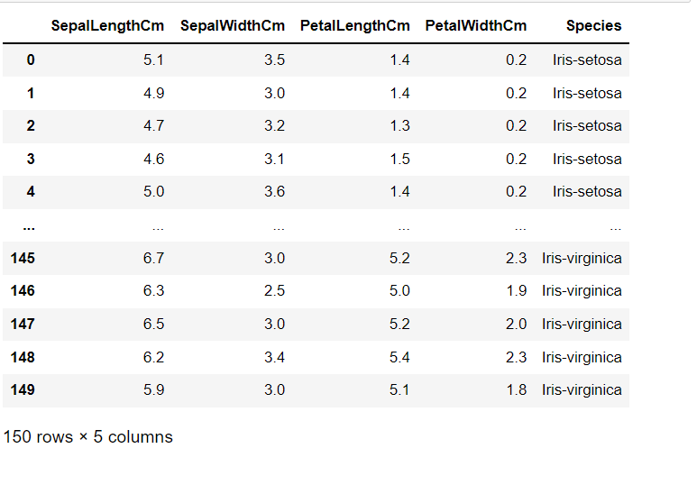
In this article of Iris Flowers Classification, we will be dealing with Logistic Regression Machine Learning Algorithm. First, we will see logistic Regression, and then we will understand the working of an algorithm with the Iris flowers dataset. We all know about Iris Dataset, and it contains features of different flower species. Independent features in this dataset are Sepal Length, Sepal Width, Petal Length, and Petal Width. All these lengths were in centimeters. And Dependent feature, which will be the output for the model, is Species. It contains the name of the species to which that particular flower with those measurements belongs.
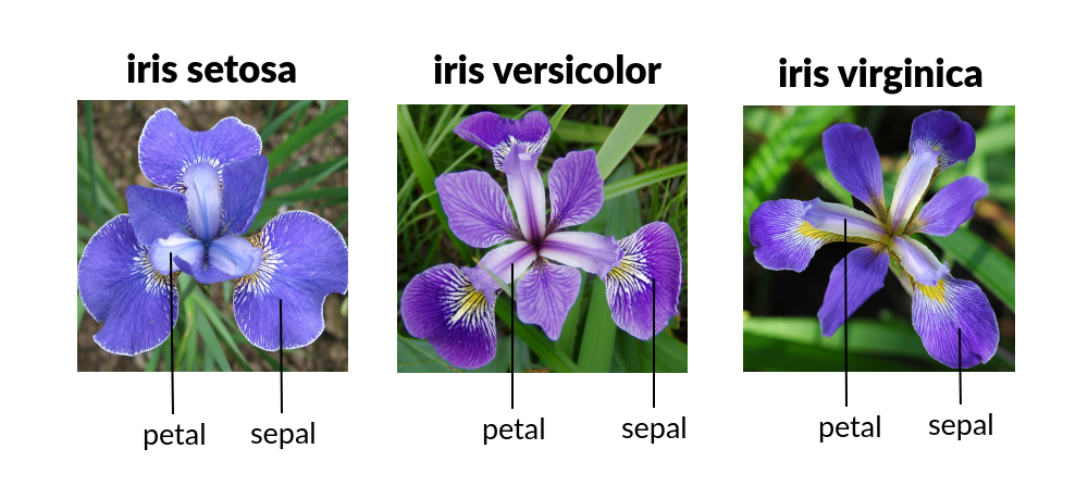
This Iris dataset is the first dataset that any data science student work on.
Before going into creating a machine learning model, let us understand Logistic Regression first.
Logistic Regression
Logistic Regression is a supervised machine learning model used mainly for categorical data, and it is a classification algorithm. It is one of the widely used algorithms for classification using machine learning. Seeing the name logistic regression, you may think it will be a regression algorithm. But the fact is that it is a classification algorithm, and it is a generalization of the linear regression model.
Logistic Regression is used to find the relationship between dependent and independent variables. This is done by using a logistic regression equation. This is a very easy to implement, understand, and also easy method to train the model.
To understand it more, think of an example of your email. You will be getting many emails, and in them, some are spam. Using this logistic Regression, we can find whether the mail is spam or ham. It will classify the emails and label them as spam or ham, like 0 or 1.
The logistic Regression model will take the mail content as input, and then it will analyze it and finally generate a label. If it is spam, it will give 1 as spam, and if it is a ham, then it will give 0, saying that it is not spam.

Working with Dataset
Before creating the model and training it, we have to preprocess the dataset. Preprocessing means converting the dataset into an understandable format before using it for any machine learning algorithms. It includes data transformation, data reduction, data cleaning, and many more.
Let us build a machine learning model using logistic Regression. For this, we will take the iris flowers dataset. This is the link for the dataset, and you can download it and store it on your local desktop.
Let us start by importing some important basic libraries.
import pandas as pd
import numpy as np
import matplotlib.pyplot as plt
import seaborn as sns
import warnings
warnings.simplefilter("ignore")
matplotlib and seaborn are used for visualizations and warnings; we can ignore all the warnings we encounter.
Import the dataset from your local desktop. Use pandas for it. Enter the path to the dataset file in the read_csv method. It will import the iris dataset.
#Import iris dataset
df=pd.read_csv(r'C:UsersAdminDownloadsIris.csv')
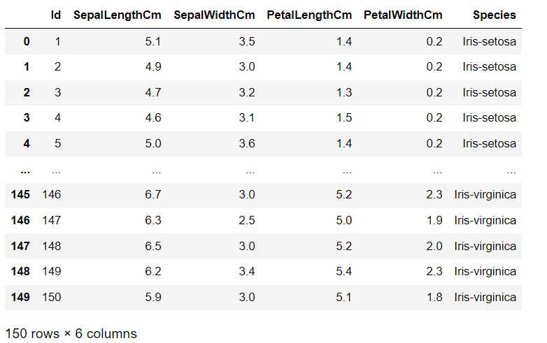
Let us view the data frame.
df
df.info()
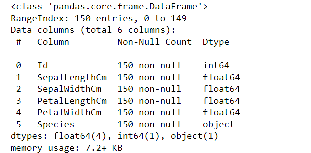
If there are any missing values, then modify them before using the dataset. For modifying you can use the fillna() method. It will fill null values.
#checking for null values
df.isnull().sum()

We can see that all values are 0. It means that there are no null values over the entire data frame.
To view the column names in the data frame, use columns
df.columns
Index(['Id', 'SepalLengthCm', 'SepalWidthCm', 'PetalLengthCm', 'PetalWidthCm',
       'Species'],
      dtype='object')
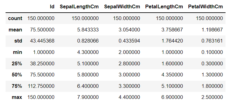
View the statistical description of the dataset.
It contains variables like count, mean, standard deviation, minimum value, maximum value, and percentiles of all the columns such as Id, Sepal length, sepal width, petal length, and petal width. Use describe() method to view it.
Python Code:
If we view the data frame, we can see two columns with the same id numbers. To delete the unwanted ID column use the drop method.
#Drop unwanted columns
df=df.drop(columns="Id")
Now view the data frame.
df
Our final data frame will look like this.
 Visualizations
View the count plot of species feature using seaborn.
df['Species'].value_counts()
Iris-setosa        50
Iris-versicolor    50
Iris-virginica     50
Name: Species, dtype: int64
sns.countplot(df['Species']);
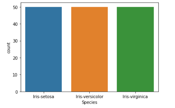 We have 150 rows in which 50 belong to Iris-setosa, 50 belong to Iris-Versicolor, and the remaining 50 belong to Iris_virginica.
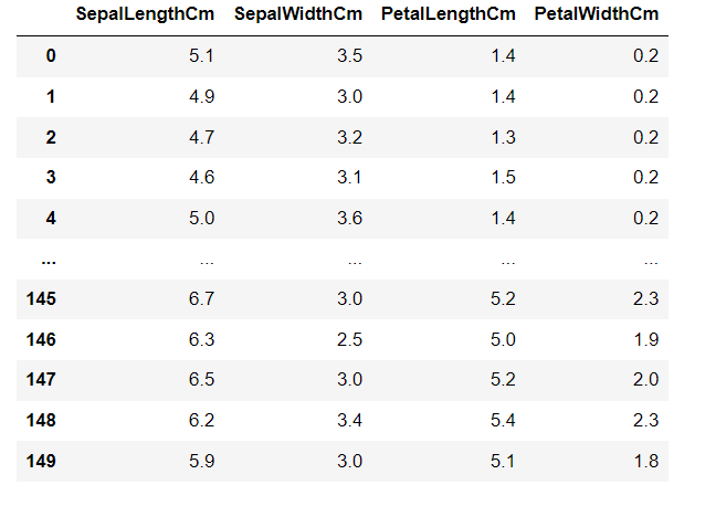
Define x and y. x contains all the input variables such as independent features, and y should contain the dependent variable which is dependent on independent variables, the output.
x=df.iloc[:,:4]
y=df.iloc[:,4]
View x
x
y
0         Iris-setosa
1         Iris-setosa
2         Iris-setosa
3         Iris-setosa
4         Iris-setosa
            ...
145    Iris-virginica
146    Iris-virginica
147    Iris-virginica
148    Iris-virginica
149    Iris-virginica
Name: Species, Length: 150, dtype: object
We can see x contains all the columns except the last column which is a dependent column and y is this dependent feature.
Split the Data Into Train and Test Datasets
To train the model and next test the model we have to split the entire dataset into train and test sets. In that, the training dataset is used to train the model and the test dataset is to test the model which has been trained with the training dataset.
Import train_test_split to split the data into train and test datasets.
from sklearn.model_selection import train_test_split
x_train,x_test,y_train,y_test=train_test_split(x,y,random_state=0)
View their shapes. Use the shape method to view.
x_train.shape
(112, 4)
x_test.shape
(38, 4)
y_train.shape
(112,)
y_test.shape
(38,)
Create the Model (Classification)
So here we are going to classify the Iris flowers dataset using logistic regression. For creating the model, import LogisticRegression from the sci-kit learn library.
from sklearn.linear_model import LogisticRegression
model=LogisticRegression()
Now train the model using the fit method. In the fit method, pass training datasets in it. x_train and y_train are the training datasets.
model.fit(x_train,y_train)
LogisticRegression()
Now predict the results using predict method.
y_pred=model.predict(x_test)
View the results now,
y_pred
array(['Iris-virginica', 'Iris-versicolor', 'Iris-setosa',
       'Iris-virginica', 'Iris-setosa', 'Iris-virginica', 'Iris-setosa',
       'Iris-versicolor', 'Iris-versicolor', 'Iris-versicolor',
       'Iris-virginica', 'Iris-versicolor', 'Iris-versicolor',
       'Iris-versicolor', 'Iris-versicolor', 'Iris-setosa',
       'Iris-versicolor', 'Iris-versicolor', 'Iris-setosa', 'Iris-setosa',
       'Iris-virginica', 'Iris-versicolor', 'Iris-setosa', 'Iris-setosa',
       'Iris-virginica', 'Iris-setosa', 'Iris-setosa', 'Iris-versicolor',
       'Iris-versicolor', 'Iris-setosa', 'Iris-virginica',
       'Iris-versicolor', 'Iris-setosa', 'Iris-virginica',
       'Iris-virginica', 'Iris-versicolor', 'Iris-setosa',
       'Iris-virginica'], dtype=object)
It will give results like this. It contains species names in the form of an array.
Find the accuracy of the model and view the confusion matrix. The accuracy score tells us how accurately the model we build will predict and the confusion matrix has a matrix with Actual values and predicted values. For that, import accuracy_score and confusion_matrix from the sci-kit learn metric library.
from sklearn.metrics import accuracy_score,confusion_matrix
confusion_matrix(y_test,y_pred)
array([[13, 0, 0],
[ 0, 15, 1],
[ 0, 0, 9]], dtype=int64)
accuracy=accuracy_score(y_test,y_pred)*100
print("Accuracy of the model is {:.2f}".format(accuracy))
Accuracy of the model is 97.37
We can see that accuracy of the model is 97.37 percent which is very accurate.
Conclusion on Classification
Flower classification is a very important, simple, and basic project for any machine learning student. Every machine learning student should be thorough with the iris flowers dataset. This classification can be done by many classification algorithms in machine learning but in our article, we used logistic regression. Overall in this article, we have seen
- Mainly we focused on Logistic Regression
- We took Iris Flowers dataset and performed a logistic regression algorithm
- Finally, it classified flowers into their species.
- And we got an accuracy of 97.37%, which shows that the model we built is very accurate.
The media shown in this article is not owned by Analytics Vidhya and is used at the Author’s discretion.


