


Introduction
This article aims to provide a basic understanding of the SVM, the optimization that is happening behind the scene, and knowledge about its parameters along with its implementation in Python.
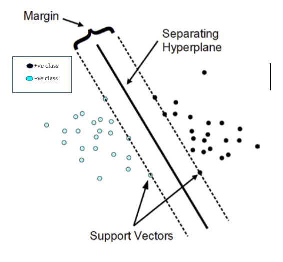
Table of Content
1. What is SVM?
2. Optimization Technique used in SVM
3. How to choose the Correct SVM
4. Hard and Soft margin SVM
5. Relation between Regularization parameter (C) and SVM
6. Other Parameters of SVM
7. Kernel -trick in SVM
8.Implementation of Support Vector Machine using Python
9. End Notes
1. What is SVM?
Support Vector Machine is a supervised learning algorithm that can be used for both classification and regression problems. It is mostly used for classification problems.
We should keep in mind that the main task of the classification problem is to find the best separating hyperplane/ Decision boundary. We can have the ‘n-1’ hyperplane which can be either linear or nonlinear.
Class labels are denoted as -1 for negative class and +1 for positive class in Support Vector Machine.
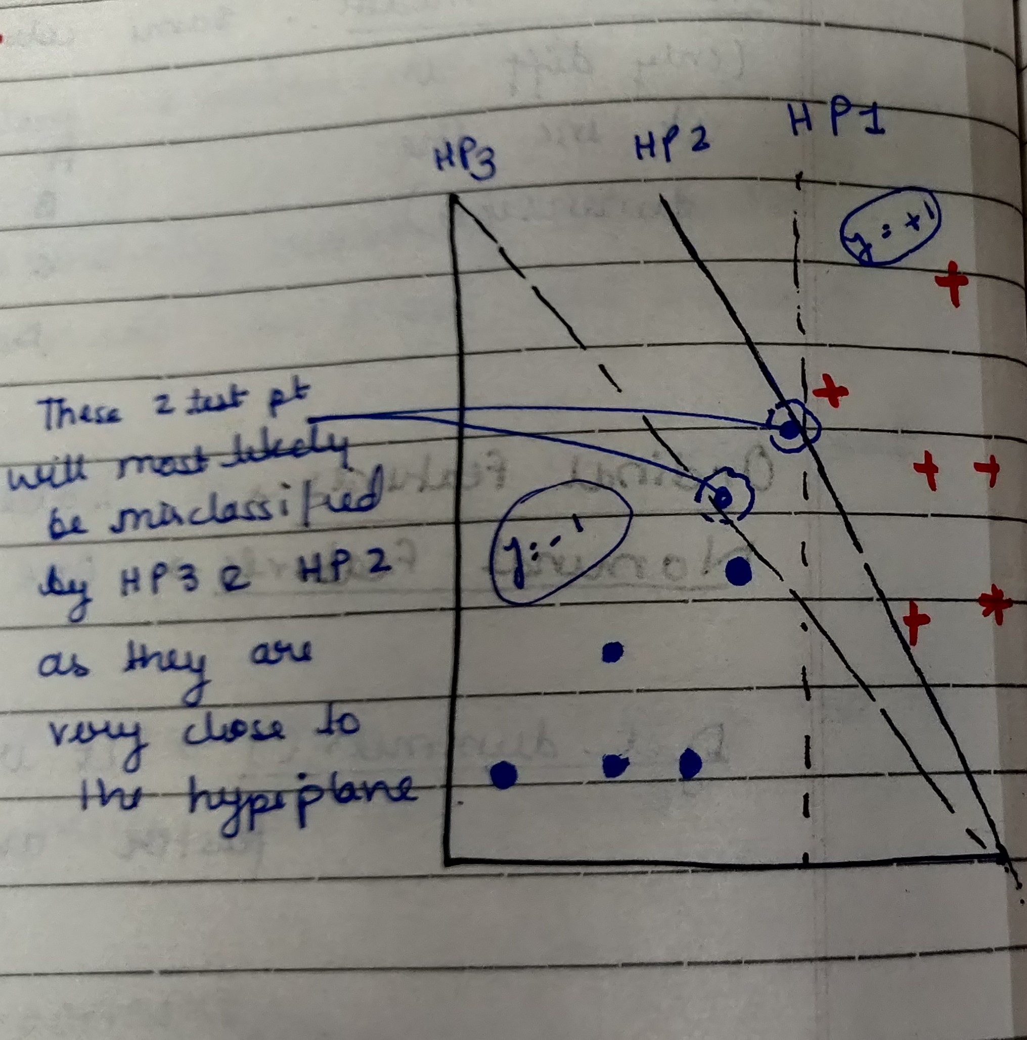
We can clearly see from the above figure that both the Hyperplane (HP2 & HP3) are not able to correctly classify the test-data points because they are very close to the hyperplane.
Such data points are called Support vectors which are simply feature values in vector form.
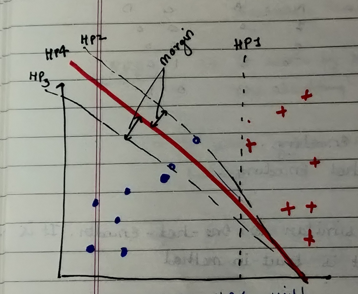
From the above figure, we can see that Hyperplane (HP4) is the best as it is able to correctly classify all the data points including support vectors.
This brings us to think what exactly are Margins?
Margins are generally defined by the closest data points (called support vectors) on either of the hyperplane
Note: Another point to note from the above figure is that the further the data points are from the margins the more correctly they are classified.
2. Optimization Technique used in SVM
The core of any Machine learning algorithm is the Optimization technique that is happening behind the scene.
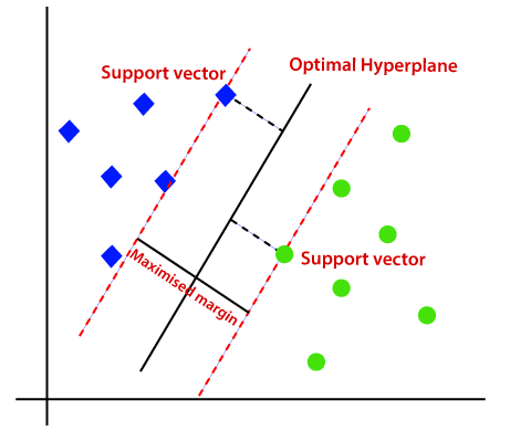
SVM maximizes the margin by learning a suitable decision boundary/decision surface/separating hyperplane.
It can be mathematically be written as:
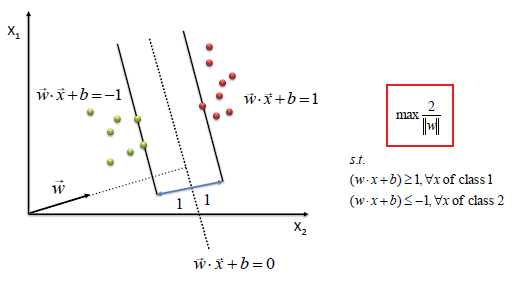
Points to note from the above Figure:
a. We can clearly see that SVM tries to maximize the margins and thus called Maximum Margin Classifier.
b. The Support Vectors will have values exactly either {+1, -1}.
c. The more negative the values are for the Green data points the better it is for classification.
d. The more positive the values are for the Red data points the better it is for classification
For more in-depth knowledge regarding the maths behind Support Vector Machine refer to this article
3. How to choose the Correct SVM
Choosing a correct classifier is really important. Let us understand this with an example.

Suppose we are given 2 Hyperplane one with 100% accuracy (HP1) on the left side and another with >90% accuracy (HP2) on the right side. Which one would you think is the correct classifier?
Most of us would pick the HP2 thinking that it because of the maximum margin. But it is the wrong answer.
But Support Vector Machine would choose the HP1 though it has a narrow margin. Because though HP2 has maximum margin but it is going against the constrain that: each data point must lie on the correct side of the margin and there should be no misclassification. This constrain is the hard constrain that Support Vector Machine follows throughout.
This brings us to the discussion about Hard and Soft SVM.
4. Hard and Soft SVM
I would like to again continue with the above example.
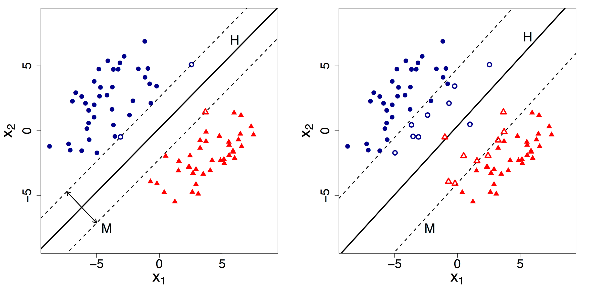
We can now clearly state that HP1 is a Hard SVM(left side) while HP2 is a Soft SVM(right side).
By default, Support Vector Machine implements Hard margin SVM. It works well only if our data is linearly separable.
Hard margin SVM does not allow any misclassification to happen.
In case our data is non-separable/ nonlinear then the Hard margin SVM will not return any hyperplane as it will not be able to separate the data. Hence this is where Soft Margin SVM comes to the rescue.
Soft margin SVM allows some misclassification to happen by relaxing the hard constraints of Support Vector Machine.
Soft margin SVM is implemented with the help of the Regularization parameter (C).
Regularization parameter (C): It tells us how much misclassification we want to avoid.
– Hard margin SVM generally has large values of C.
– Soft margin SVM generally has small values of C.
5. Relation between Regularization parameter (C) and SVM
Now that we know what the Regularization parameter (C) does. We need to understand its relation with Support Vector Machine.
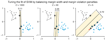
– As the value of C increases the margin decreases thus Hard SVM.
– If the values of C are very small the margin increases thus Soft SVM.
– Large value of C can cause overfitting therefore we need to select the correct value using Hyperparameter Tuning.
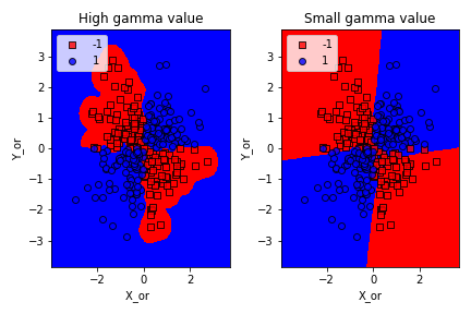
6. Other Parameters of SVM
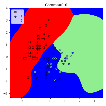
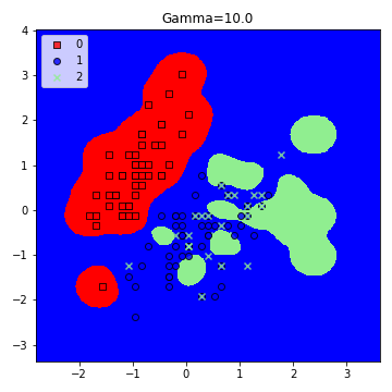
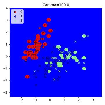
Other significant parameters of Support Vector Machine are the Gamma values. It tells us how much will be the influence of the individual data points on the decision boundary.
– Large Gamma: Fewer data points will influence the decision boundary. Therefore, decision boundary becomes non-linear leading to overfitting
– Small Gamma: More data points will influence the decision boundary. Therefore, the decision boundary is more generic.
7. Kernel -trick in SVM
Support Vector Machine deals with nonlinear data by transforming it into a higher dimension where it is linearly separable. Support Vector Machine does so by using different values of Kernel. We have various options available with kernel like, ‘linear’, “rbf”, ”poly” and others (default value is “rbf”). Here “rbf” and “poly” are useful for non-linear hyper-plane.
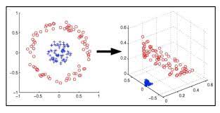
From the above figure, it is clear that choosing the right kernel is very important in order to get the correct results.
8.Implementation of SVM using Python
For this part, I will be using the Iris dataset.
1. Load the libraries and the dataset.
Python Code:
2. I have created a Decision Boundary function for better understanding.
def decision_boundary(X,y,model,res,test_idx=None):
    markers=['s','o','x']
    colors = ('red', 'blue', 'lightgreen', 'gray', 'cyan')
    colormap=ListedColormap(colors[:len(np.unique(y))])
    x_min,x_max=X[:,0].min()-1,X[:,0].max()+1
    y_min,y_max=X[:,1].min()-1,X[:,1].max()+1
    xx,yy=np.meshgrid(np.arange(x_min,x_max,res),np.arange(y_min,y_max,res))
    z=model.predict(np.c_[xx.ravel(), yy.ravel()])
    zz=z.reshape(xx.shape)
    plt.pcolormesh(xx,yy,zz,cmap=colormap)

    for idx,cl in enumerate(np.unique(y)):
        plt.scatter(X[y==cl,0],X[y==cl,1],c=colors[idx],cmap=plt.cm.Paired, edgecolors='k',marker=markers[idx],label=cl,alpha=0.8)
3. Split the dataset and Standardize the data
from sklearn.model_selection import train_test_split
from sklearn.preprocessing import StandardScaler
X_train,X_test,y_train,y_test=train_test_split(X,Y,test_size=0.3)
scaler=StandardScaler()
scaler.fit(X_train)
X_train_new=scaler.transform(X_train)
X_test_new=scaler.transform(X_test)
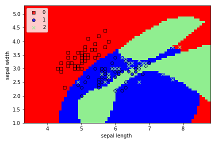
4. I have implemented the Soft & Hard SVM by experimenting with high and low values of C
model=SVC(C=10**10)model.fit(X_train,y_train) # Hard SVM
decision_boundary(np.vstack((X_train,X_test)),np.hstack((y_train,y_test)),model,0.08,test_idx=None)
plt.xlabel('sepal length ')
plt.ylabel('sepal width ')
plt.legend(loc='upper left')
plt.tight_layout()
plt.show()
model=SVC(C=100)  # Soft SVM
model.fit(X_train,y_train)
decision_boundary(np.vstack((X_train,X_test)),np.hstack((y_train,y_test)),model,0.08,test_idx=None)
plt.xlabel('sepal length ')
plt.ylabel('sepal width ')
plt.legend(loc='upper left')
plt.tight_layout()
plt.show()
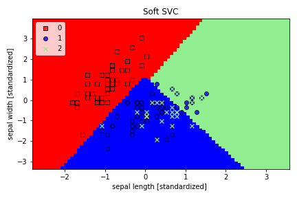
We can clearly see that Soft SVM allows for some misclassification, unlike Hard SVM.
5. Experimenting with gamma values.
plt.figure(figsize=(5,5))
model = SVC(kernel='rbf', random_state=1, gamma=1.0, C=10.0)
model.fit(X_train_new,y_train)
decision_boundary(np.vstack((X_train_new,X_test_new)),np.hstack((y_train,y_test)),model,0.02,test_idx=None)
plt.title('Gamma=1.0')
plt.legend(loc='upper left')
plt.tight_layout()
plt.show()
plt.figure(figsize=(5,5))
model = SVC(kernel='rbf', random_state=1, gamma=10.0, C=10.0)
model.fit(X_train_new,y_train)
decision_boundary(np.vstack((X_train_new,X_test_new)),np.hstack((y_train,y_test)),model,0.02,test_idx=None)
plt.title('Gamma=10.0')
plt.legend(loc='upper left')
plt.tight_layout()
plt.show()
plt.figure(figsize=(5,5))
model = SVC(kernel='rbf', random_state=1, gamma=100.0, C=10.0)
model.fit(X_train_new,y_train)
decision_boundary(np.vstack((X_train_new,X_test_new)),np.hstack((y_train,y_test)),model,0.02,test_idx=None)
plt.title('Gamma=100.0')
plt.legend(loc='upper left')
plt.tight_layout()
plt.show()
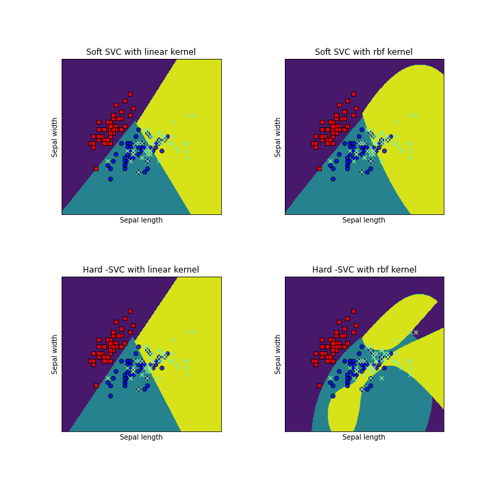
6. Implementing the Kernel -trick along with experimenting with the values of C.
For this part, I have created a function for creating sub-plots along with Decision-Boundary.
def create_mesh(x,y,res=0.02):
    x_min,x_max=x.min()-1,x.max()+1
    y_min,y_max=y.min()-1,y.max()+1
    xx,yy=np.meshgrid(np.arange(x_min,x_max,res),np.arange(y_min,y_max,res))
    return xx,yy
def create_contours(ax,clf,xx,yy,**parameters):
    z=clf.predict(np.c_[xx.ravel(),yy.ravel()])
    zz=z.reshape(xx.shape)
    out = ax.contourf(xx, yy, zz)
    return out
## Creating the sub-plots
models = (svm.SVC(kernel='linear', C=1.0),
          svm.SVC(C=1.0),SVC(C=10**10,kernel='linear'),SVC(C=10**10,kernel='rbf'))
models = (clf.fit(X_train, y_train) for clf in models)
# title for the plots
titles = ('Soft SVC with linear kernel',
          'Soft SVC with rbf kernel', 'Hard -SVC with linear kernel','Hard -SVC with rbf kernel')
# Set-up 2x2 grid for plotting.
fig, sub = plt.subplots(2, 2,figsize=(10,10))
plt.subplots_adjust(wspace=0.4, hspace=0.4)
xx,yy=create_mesh(X[:,0], X[:,1])
for clf, title, ax in zip(models, titles, sub.flatten()):
    markers=['s','o','x']
    colors = ('red', 'blue', 'lightgreen', 'gray', 'cyan')
    colormap=ListedColormap(colors[:len(np.unique(Y))])
    create_contours(ax, clf, xx, yy,cmap=colormap)
    for idx,cl in enumerate(np.unique(Y)):
        ax.scatter(X[Y==cl,0],X[Y==cl,1],c=colors[idx],cmap=colormap, edgecolors='k',marker=markers[idx],label=cl,alpha=0.8)
        ax.set_xlim(xx.min(), xx.max())
        ax.set_ylim(yy.min(), yy.max())
        ax.set_xlabel('Sepal length')
        ax.set_ylabel('Sepal width')
        ax.set_xticks(())
        ax.set_yticks(())
        ax.set_title(title)
plt.show()

9. End Notes
In this article, we looked at the Support Vector Machine in detail. I have discussed in detail the important concepts which are needed for proper understanding along with its implementation in Python. I hope you like this article, if you do please like and share.
For the whole code, implementation refer to my Github Repository
Dishaa Agarwal My interests lie in the field of Machine Learning and Data Science. Enthusiasm to learn new skills is always present in me.