This article was published as a part of the Data Science Blogathon.
Introduction
This article introduces the concept of Manifold Learning. It also discusses one of its techniques- LLE (Locally Linear Embedding) and its implementation.
The curse of dimensionality
A large number of machine learning datasets involve thousands and sometimes millions of features. These features can make training very slow. In addition, there is plenty of space in high dimensions making the high-dimensional datasets very sparse, as most of the training instances are quite likely to be far from each other. This increases the risk of overfitting since the predictions will be based on much larger extrapolations as compared to those on low-dimensional data. This is called the curse of dimensionality.
There are two main approaches for dimensionality reduction: Projection and Manifold Learning. Here, we will focus on the latter.
What is Manifold Learning?
What is a manifold?
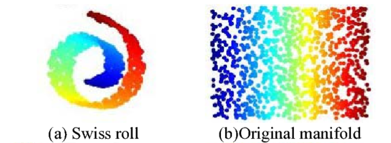
A two-dimensional manifold is any 2-D shape that can be made to fit in a higher-dimensional space by twisting or bending it, loosely speaking.
What is the Manifold Hypothesis?
“The Manifold Hypothesis states that real-world high-dimensional data lie on low-dimensional manifolds embedded within the high-dimensional space.”
In simpler terms, it means that higher-dimensional data most of the time lies on a much closer lower-dimensional manifold. The process of modeling the manifold on which training instances lie is called Manifold Learning.

Ref: Figure 2, Gu, Rui-jun, and Wenbo Xu. “An Improved Manifold Learning Algorithm for Data Visualization.” 2006 International Conference on Machine Learning and Cybernetics (2006): 1170-1173.
Locally Linear Embedding (LLE)
Locally Linear Embedding (LLE) is a Manifold Learning technique that is used for non-linear dimensionality reduction. It is an unsupervised learning algorithm that produces low-dimensional embeddings of high-dimensional inputs, relating each training instance to its closest neighbor.
How does LLE work?
For each training instance x(i), the algorithm first finds its k nearest neighbors and then tries to express x(i) as a linear function of them. In general, if there are m training instances in total, then it tries to find the set of weights w which minimizes the squared distance between x(i) and its linear representation.
So, the cost function is given by

where wi,j =0, if j is not included in the k closest neighbors of i.
Also, it normalizes the weights for each training instance x(i),

Finally, each high-dimensional training instance x(i) is mapped to a low-dimensional (say, d dimensions) vector y(i) while preserving the neighborhood relationships. This is done by choosing d-dimensional coordinates which minimize the cost function,

Here the weights wi,j are kept fixed while we try to find the optimum coordinates y(i)
Implementation using scikit-learn
The following code is used to implement LLE using scikit-learn’s LocallyLinearEmbedding class:
X_transformed=lle.fit_transform(X)
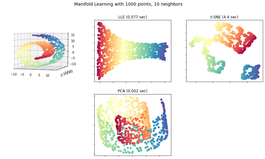
Now, we will compare LLE with PCA and t-SNE on the swiss roll dataset.
#Importing the required libraries
from collections import OrderedDict
from functools import partial
from time import time
import matplotlib.pyplot as plt
from mpl_toolkits.mplot3d import Axes3D
from matplotlib.ticker import NullFormatter
from sklearn import manifold, datasets
from sklearn.decomposition import PCA
#This import is needed to silence pyflakes
Axes3D
#Then we load the swiss roll dataset
n_points = 1000
X, color = datasets.make_swiss_roll(n_points, random_state=0)
n_neighbors = 10
n_components = 2
# Creating the plot
fig = plt.figure(figsize=(15, 8))
fig.suptitle("Manifold Learning with %i points, %i neighbors"
             % (1000, n_neighbors), fontsize=14)
# Adding 3d scatter plot
ax = fig.add_subplot(231, projection='3d')
ax.scatter(X[:, 0], X[:, 1], X[:, 2], c=color, cmap=plt.cm.Spectral)
ax.view_init(4, -72)
# Making a dictionary 'methods' containing LLE, t-SNE and PCA
LLE = partial(manifold.LocallyLinearEmbedding,
              n_neighbors, n_components, eigen_solver='auto')
methods = OrderedDict()
methods['LLE'] = LLE(method='standard')
methods['t-SNE'] = manifold.TSNE(n_components=n_components, init='pca',
                                 random_state=0)
methods['PCA']=PCA(n_components=2)
# Plotting the results
for i, (label, method) in enumerate(methods.items()):
    t0 = time()
    Y = method.fit_transform(X)
    t1 = time()
    print("%s: %.2g sec" % (label, t1 - t0))
    ax = fig.add_subplot(2, 3, 2 + i+(i>1))
    ax.scatter(Y[:, 0], Y[:, 1], c=color, cmap=plt.cm.Spectral)
    ax.set_title("%s (%.2g sec)" % (label, t1 - t0))
    ax.xaxis.set_major_formatter(NullFormatter())
    ax.yaxis.set_major_formatter(NullFormatter())
    ax.axis('tight')
plt.show()
Output: We get the following plot:

End Notes
The use of manifold learning is based on the assumption that our dataset or the task which we are doing will be much simpler if it is expressed in lower dimensions. But this may not always be true. So, dimensionality reduction may reduce training time but whether or not it will lead to a better solution depends on the dataset.
Conclusion
In this article, we introduced the concept of Manifold Learning and also discussed one of its techniques-LLE. Then we saw its python implementation and also compared LLE with t-SNE and PCA on the swiss roll dataset.
References:
- Roweis, S. T., & Saul, L. K. (2000).Nonlinear dimensionality reduction by locally linear embedding. Science(New York, N.Y.), 290(5500), 2323–2326.
- Manifold Hypothesis Definition | Deep AI
- https://scikit-learn.org/stable/modules/generated/sklearn.manifold.LocallyLinearEmbedding.html#sklearn.manifold.LocallyLinearEmbedding
- https://scikit-learn.org/stable/auto_examples/manifold/plot_compare_methods.html#sphx-glr-auto-examples-manifold-plot-compare-methods-py
Hope you enjoyed reading this article! 🙂
About the author
I am Isha Sharma, currently pursuing B.Tech from the Indian Institute of Technology Kharagpur. I am passionate about data science and deep learning.
The media shown in this article are not owned by Analytics Vidhya and is used at the Author’s discretion.


