Identifying the Source of Bootstrap Methodology’s Power

This article was published as a part of the Data Science Blogathon

From where we stand the rain seems random. If we could stand somewhere else, we would see the order in it.
– Tony Hillerman, Coyote Waits

Shuffling is the only thing which Nature cannot undo.
– Arthur Eddington

Abstract:

Bootstrap is a pretty common methodology in the field of machine learning. Today we will try to better understand what it does and why is it efficient. We will try to find “the source of the power of bootstrap methodology“. The above two quotes capture the essence of this strength – the order behind apparent randomness, and the power of shuffling. By the end of this article, we expect to understand why bootstrap works and when it might not.

Sections:

We will divide this article into the following sections –

• The need for bootstrap
• A brief overview of bootstrap
• Strategy to evaluate bootstrap
• Effectiveness of bootstrap
• A major challenge of bootstrap methodology
• Conclusion

The need for bootstrap:

Why is bootstrap necessary? We need a background of this first. So let’s have a quick overview.

All machine learning methods, at least the statistical learning ones, essentially have the same approach – choose a model and tune the parameters to best fit the real world. Now the parameter values will vary from one run to the other based on the different training sets they choose. Hence the parameters have an uncertainty attached to them. Accordingly, it is a prevalent practice, and a good one actually, to quote a confidence interval for the parameter values. These confidence intervals become very essential when one does inferential tasks – like hypothesis testing to determine how relevant a certain feature is in the context of the analysis.

How are these confidence intervals constructed?

Normally by making some logical, time-tested assumptions and performing some mathematical gymnastics based on those assumptions. This used to be and still is, the domain of statisticians. For e.g., in linear regression model y_i=a+bx_i+e_i, various assumptions are made for e_i such as being generated from a 0 mean distribution of e, e_i being uncorrelated to std(e), etc. These assumptions help in constructing the confidence interval around the estimates for a and b.

However, for real-world scenarios such assumptions rarely hold. Besides, most machine learning models, unlike linear regression, are too complex to allow for such analytical tactics. So what’s the way forward for the machine learning community.

We take the brute-force approach, which will be called the naive approach from now on. We take a number of training sets, fit the model to each dataset to get a sequence of parameter values. The standard deviation of this sequence of parameter values helps us construct the confidence intervals.

Pretty simple, but unfortunately almost never done.

We never have so many training sets at our disposal in the real world. It is in this context that bootstrap becomes relevant.

Source: Google images

The term “bootstrapping” originated with a phrase in use in the 18th and 19th century: “to pull oneself up by one’s bootstraps.” Back then, it referred to an impossible task. Today it refers more to the challenge of making something out of nothing.

A brief overview of bootstrap:

Taking multiple training sets of a given size – is the step that bootstrap tries to replicate. We have one training set of say 100 samples. We need to randomly choose (with replacement) 100 samples from this training set to get another training set. In this way, we can get as many training sets as we need. The rest of the approach remains the same as above.

So bootstrap essentially assumes that by resampling one training set to produce many training set replicas we can replicate the event of having multiple training sets at our disposal.

Say we have one set of three observations – (1,4,9). We need two more such sets. Bootstrap resamples from this very training set to get, (1,1,9) and (4,9,1) say.

It is the effectiveness of this assumption that we will verify.

Strategy to evaluate bootstrap:

We first need to understand what is the relationship of one training set to another. They have some similarities on account of being generated from the same population. But they also differ because of the natural tendency of one sample to vary from another. We need to decide upon a few features that capture the similarities and dissimilarities.

1. The mean, standard deviation, quartile ranges of a training set are something that is characteristics of the population. All training sets of a certain size derived from the same population will show
   nearly the same values for these parameters.
2. The distribution of the training set is something that varies from one to another. If a histogram plot is made for the training sets, how much one plot varies from the other will indicate this variance.
   To quantify this we decide upon a metric – the sum of squares of the difference of histogram bars – let’s call it the dissimilarity metric.

If training sets generated by naive and bootstrap approaches respectively show close enough values for the above metrics then we will consider bootstrap to be a possible replacement for the naive approach.

Effectiveness of bootstrap:

The training set was generated using a uniform distribution between (0, 10.0). The training set size was 1000 and 100 such training sets were generated for the naive and bootstrap approaches respectively.

The following are the distribution of the 100 –

• means
• standard deviations (STDs)
• 0, 25, 50, 75, and 100 percentile marks
• dissimilarity metric

for both approaches.

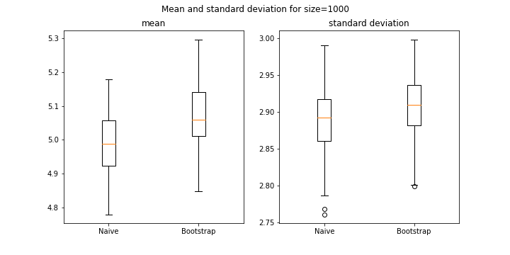
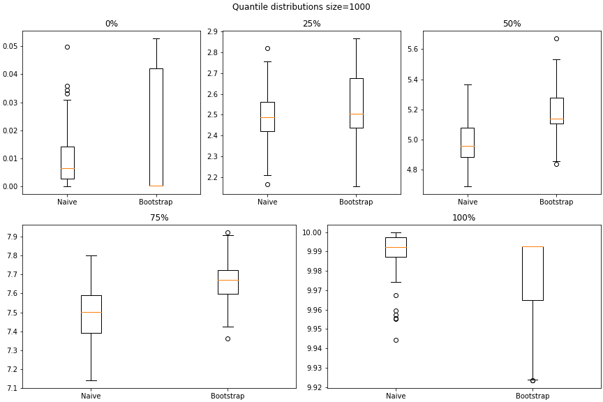
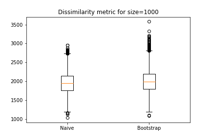
For mean, STD, and quantile distributions the difference between the two approaches are within one decimal place. For dissimilarity metricss, they are pretty similar.

A major challenge of bootstrap methodology:

Suppose we have a training set (1, 2) with mean 1.5. Bootstrap generates two more training sets (1, 1) and (2, 2) each with a probability of 25% and means 1 and 2 respectively. Naive method gives two further training sets (1, 3) and (4, 5) respectively.

It is obvious that as training set size becomes small or does not cover the entire range of possible inputs bootstrap becomes inefficient. To demonstrate that, the same experiment as above was repeated, but with training set size of 10. The results are as follows –

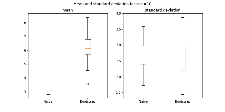
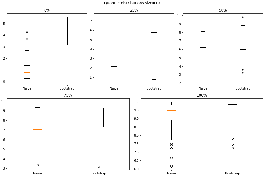
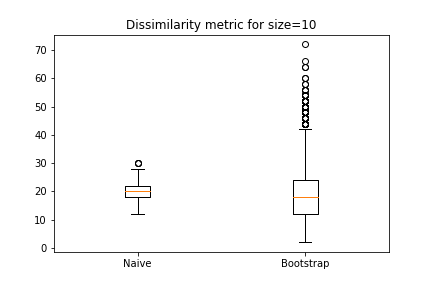
The y-axis scales make it clear that the differences have gone up by ~10 times.

So small training sets, as compared to the range of sample values, become a challenge for bootstrap.

Conclusion:

Hence, shuffling is the strength by which bootstrap aims to replicate the randomness of nature.

That’s what the card players did all along. A small deck of cards might lead to a bad hand though.

Source: Google images

PS:

The codes used to generate the above simulations and plots can be found in my github repository.

About the author:

I am an IT professional, enthusiastic about machine learning, mathematics and writing insightful blogs on similar topics. Please check out my linkedin profile for similar updates.

Anirban Chakraborty

04 Jul 2021