This article was published as a part of the Data Science Blogathon.
Introduction
Almost every data scientist must have encountered the data for which they need to perform imbalanced binary classification. Imbalanced data means the number of rows or frequency of data points of one class is much more than the other class. In other words, the ratio of the value counts of classes is much higher. Such data set is known as an imbalanced dataset in which the class having more data points is the majority class and the other is the minority class.
The imbalance makes the classification more challenging. Whenever we build a classifier with such data, it works well with the majority class but gives a poor performance with the minority class. Although, the model performance concerning the minority class matters the most. Some Machine Learning algorithms are more sensitive toward imbalanced data, such as Logistic Regression and Support Vector Machine. However, some algorithms tackle this issue themselves, such as Random Forest and XGBoost.
Now, the question comes of how to help algorithms that do not tackle imbalanced data on their own?
That’s when the sampling technique comes to save us and deal with imbalanced data.
There are two sampling techniques available to handle the imbalanced data:
- Under Sampling
- Over Sampling
This article will cover these techniques along with their implementation in Python. So get ready for some buggy code battle.
Sampling
The idea behind sampling is to create new samples or choose some records from the whole data set.
At first, we will load the imbalanced dataset using Python and Pandas. For this task, we are using the AID362_train from Bioassay datasets available on Kaggle.
Let’s create a new anaconda environment (optional but recommended) and open our Jupyter Notebook or any IDE you want to use, go for it.
Then import the necessary libraries as shown in the code snippet.
import pandas as pd
import numpy as np
import imblearn
import matplotlib.pyplot as plt
import seaborn as sns
Now read the CSV file into the notebook using pandas and check the first five rows of the data frame.
train = pd.read_csv('AID362red_train.csv')
train.head()
Then check the class frequency using value_counts and find the class distribution ratio.
train['Outcome'].value_counts()
inactive = len(train[train['Outcome'] == 'Inactive'])
active = len(train[train['Outcome'] == 'Active'])
class_distribution_ratio = inactive/active
The data is highly imbalanced, with a ratio of 70:1 for the majority to the minority class. Now, let’s tackle this imbalanced data using various Undersampling techniques first.
Under Sampling
Under Sampling techniques helps in balancing the class distribution for skewed class distribution. Imbalanced class distribution has more examples from one or more classes (majority class) and few examples belonging to minority classes.
Undersampling techniques eliminate some examples from the training data set belonging to the majority class. It is to better balance the class distribution by reducing the skewness of 1:80 to 1:5 or 1:1. Under-sampling is used along with the conjunction of an Over-sampling method. These techniques’ combination often gives better results than using any of these alone.
The basic Undersampling technique removes the examples randomly from the majority class, referred to as ‘randomundersampling.’ Although this is simple and sometimes effective too, there is a risk of losing useful or important information that could determine the decision boundary between the classes.
Therefore, there is a need for a more heuristic approach that can choose examples for non-deletion and redundant examples for deletion.
Fortunately, some undersampling techniques do use such heuristics. These we will discuss in the upcoming sections.
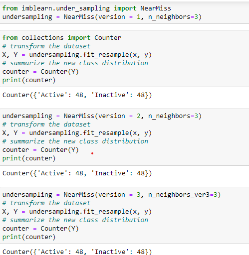
Near Miss Undersampling
This technique selects the data points based on the distance between majority and minority class examples. It has three versions of itself, and each of these considers the different neighbors from the majority class.
- Version 1 keeps examples with a minimum average distance to the nearest records of the minority class.
- Version 2 selects rows with a minimum average distance to the furthest records of the minority class.
- Version 3 keeps examples from the majority class for each closest record in the minority class.
Among these, version 3 is more accurate since it considers examples of the majority class that are on the decision boundary.
Let’s implement each of these with Imblearn and Python.
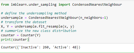
Condensed Nearest Neighbor (CNN) Undersampling
This technique aspires to a subset of a collection of samples that minimizes the model loss. These examples are stores in a store that then consists of examples from the minority class and incorrectly classified examples from the majority class.
Tomek Links Undersampling
This technique is the modified version of CNN in which the redundant examples get selected randomly for deletion from the majority class. These examples are rather internal than near the decision boundary.
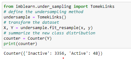
Since it uses redundant examples, it barely balances the data.
Edited Nearest Neighbors Undersampling
This technique uses the nearest neighbors approach and deletes according to the misclassification of the samples. It computes three nearest neighbors for each instance. If the example of a majority class and misclassified by these three neighbors. Then it removes that instance.
If the instance is of the minority class and misclassified by the three nearest neighbors, then its neighbors from the majority class are removed.
One-Sided Selection Undersampling
This technique combines Tomek Links and the CNN rule. Tomek links remove the noisy and borderline examples, whereas CNN removes the distant examples from the majority class.
 Neighborhood Cleaning Undersampling
This approach is a combination of CNN and ENN techniques. Initially, it selects all the minority class examples. Then ENN identifies the ambiguous samples to remove from the majority class. Then CNN deletes the misclassified examples against the store if the majority class has more than half of the minority class examples.
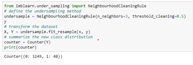
We have seen some undersampling techniques. Let’s dive into Oversampling techniques to handle the imbalanced data.
Oversampling
Unlike Undersampling, which focuses on removing the majority class examples, Oversampling focuses on increasing minority class samples.
We can also duplicate the examples to increase the minority class samples. Although it balances the data, it does not provide additional information to the classification model.
Therefore synthesizing new examples using an appropriate technique is necessary. Here SMOTE comes into the picture.
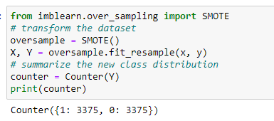
SMOTE
SMOTE stands for Synthetic Minority Oversampling Technique.
SMOTE selects the nearest examples in the feature space, then draws a line between them, and at a point along the line, it creates a new sample.
“First of all, SMOTE picks an instance randomly from the minority class. Then it finds its k nearest neighbors from the minority class itself. Then one of the neighbors gets chosen randomly and draws the line between these two instances. Then new synthetic examples are generated using a convex combination of these two instances.”
Borderline-SMOTE
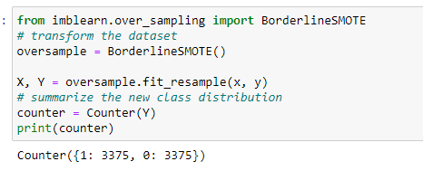
This SMOTE extension selects the minority class instance that is misclassified with a k-nearest neighbor (KNN) classifier. Since borderline or distant examples are more tend to misclassified.
Borderline-SMOTE SVM
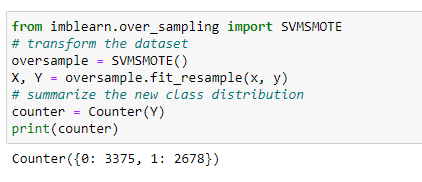
This method selects the misclassified instances of Support Vector Machine (SVM) instead of KNN.
Adaptive Synthetic Sampling (ADASYN)
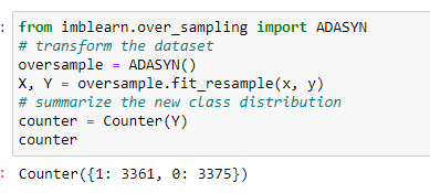
This approach works according to the density of the minority class instances. Generating new samples is inversely proportional to the density of the minority class samples.
It generates more samples in the feature space region where minority class examples density is low or none and fewer samples in the high-density space.
Conclusion
Thus all the techniques, to handle imbalanced data, along with their implementation are covered. After analyzing all the outputs we can say that oversampling tends to work better in handling the imbalanced data. However, it is always recommended to use both, Undersampling and Oversampling to balance the skewness of the imbalanced data. Let’s discuss some key takeaways from this article:
- Imbalanced data affects the performance of the classification model.
- Thus to handle the imbalanced data, Sampling techniques are used.
- There are two types of sampling techniques available: Undersampling and Oversampling.
- Undersampling selects the instances from the majority class to keep and delete.
- Oversampling generates the new synthesis examples from the minority class using neighbors and density distribution criteria.
- It is recommended to use both techniques altogether to get better results for the model performance.
Dataset Link: https://www.kaggle.com/code/stevenkoenemann/aid-362-red-neural-network/data?select=AID362red_train.csv
The media shown in this article is not owned by Analytics Vidhya and is used at the Author’s discretion.


