This article was published as a part of the Data Science Blogathon.
Introduction
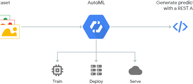
H2O is a fully open-source, distributed in-memory machine learning platform with linear scalability. H2O supports the most widely used statistical & machine learning algorithms, including gradient boosted machines, generalized linear models, deep learning, and many more. AutoML is a function in H2O that automates the process of building a large number of models, with the goal of finding the “best” model without any prior knowledge or effort by the Data Scientist.
The current version of H2O AutoML trains and cross-validates a default Random Forest, an Extremely-Randomized Forest, a random grid of Gradient Boosting Machines (GBMs), a random grid of Deep Neural Nets, a fixed grid of GLMs, and then trains two Stacked Ensemble models at the end. One ensemble contains all the models (optimized for model performance), and the second ensemble contains just the best performing model from each algorithm class/family (optimized for production use).
Automated Machine Learning (AutoML) is the process of automating the end-to-end process of applying machine learning to real-world problems. In a typical machine learning application, the typical stages (and sub-stages) of work are the following:
- Data preparation
- data pre-processing
- feature engineering
- feature extraction
- feature selection
- Model selection
- Hyperparameter optimization (to maximize the performance of the final model)
Many of these steps are often beyond the abilities of non-experts. H2O AutoML was proposed as an artificial intelligence-based solution to the ever-growing challenge of applying machine learning.
Start H2O
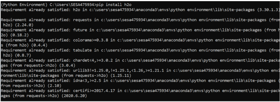
Import the h2o Python module and H2OAutoML class and initialize a local H2O cluster. The H2O library can simply be installed by running pip. Next, import the libraries in your jupyter notebook. Here, I have imported pandas for data preprocessing work.
pip install h2o
import pandas as pd
import h2o
from h2o.automl import H2OAutoML
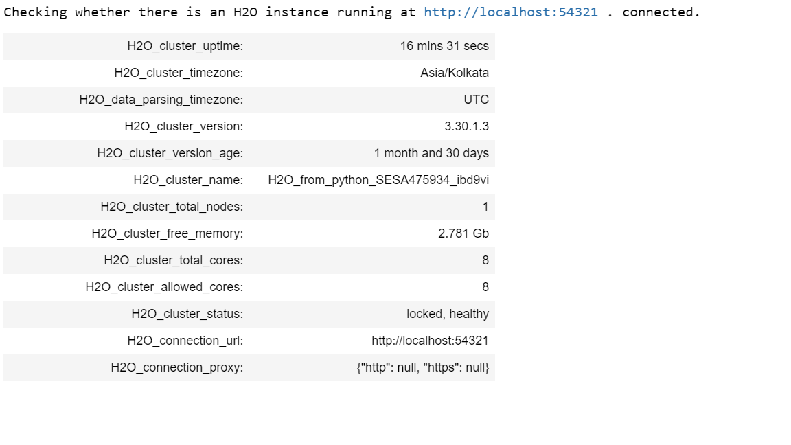
Initiate H20, the specified arguments (nthreads and max_mem_size) are optional.
h2o.init(
    nthreads=-1,     # number of threads when launching a new H2O server
    max_mem_size=12  # in gigabytes
)
Load Data
train = h2o.import_file("C:\Burnout_Rate_Prediction\dataset\train.csv")
test = h2o.import_file("C:\Burnout_Rate_Prediction\dataset\test.csv")
Data Processing
Convert H2O frame to Pandas dataframe. This is done so that data operations can be easily done. Also, drop rows that have missing values.
train_as_df = h2o.as_list(train,use_pandas=True)
train_as_df = train_as_df[train_as_df['Burn Rate'].notna()]
train_as_df = train_as_df[train_as_df['Mental Fatigue Score'].notna()]
train_as_df = train_as_df[train_as_df['Resource Allocation'].notna()]
train_as_df.head(2)

Check for any missing values. In this case, there are no missing values to be treated.
round((train_as_df.isnull().sum() * 100/ len(train_as_df)),2).sort_values(ascending=False)

Convert Pandas data frame back to H2O frame to continue with further processing.
train = h2o.H2OFrame(train_as_df)

Build Model
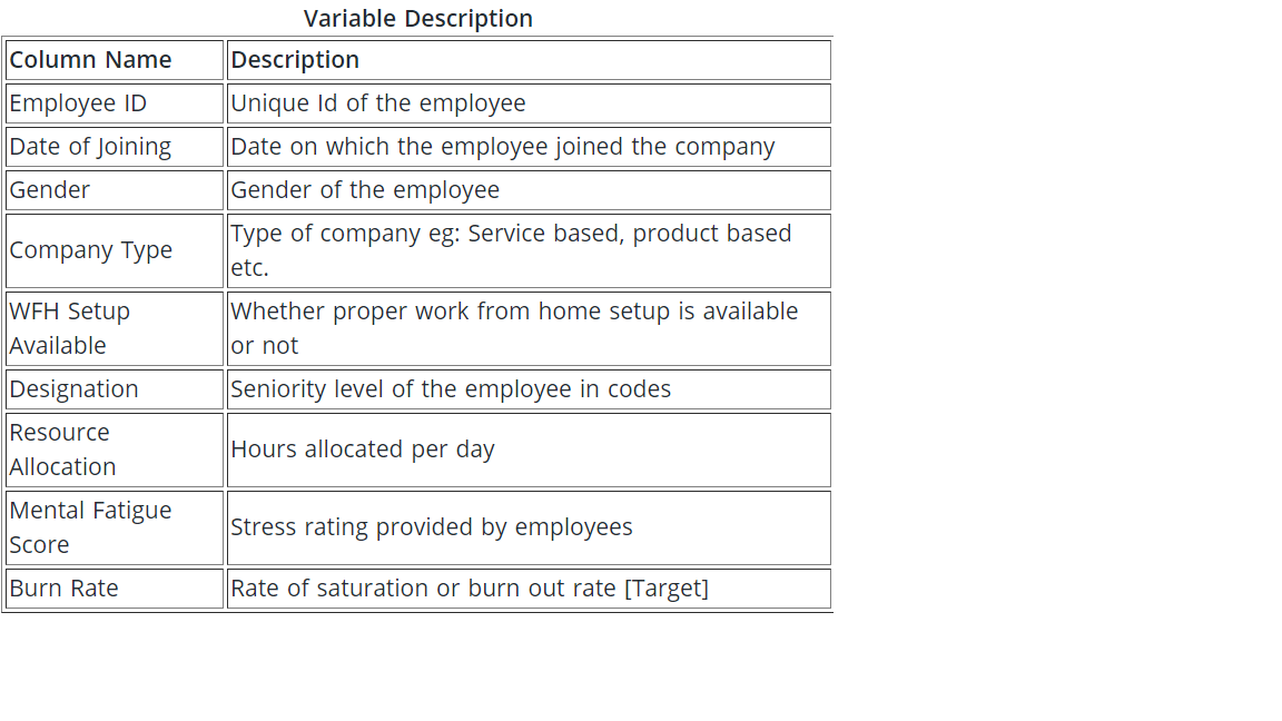
First, identify predictors and response variables. Since we are predicting ‘Burn Rate’ among employees so it will be the response variable. The remaining variables in the dataframe will form the predictor variables.
x = train.columns
y = "Burn Rate"
x.remove(y)
Run AutoML for 10 base models (limited to 1-hour max runtime by default). The ‘max_models’ argument specifies the number of individuals (or “base”) models and does not include any ensemble models that can be trained separately.
aml = H2OAutoML(max_models=10, seed=1)
aml.train(x=x, y=y, training_frame=train)

View LeaderBoard
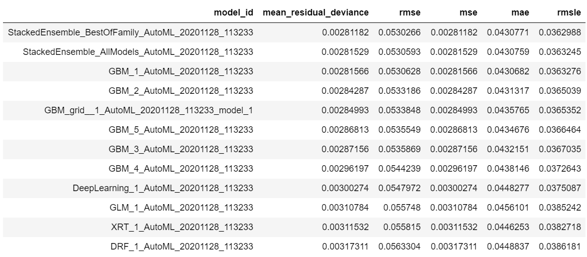
Next, we will view the AutoML Leaderboard. Since we did not specify a leaderboard_frame in the H2OAutoML.train() method for scoring and ranking the models, the AutoML leaderboard uses cross-validation metrics to rank the models.
A default performance metric for each machine learning task (binary classification, multiclass classification, regression) is specified internally and the leaderboard will be sorted by that metric. In the case of binary classification, the default ranking metric is Area Under the ROC Curve (AUC). In the future, the user will be able to specify any of the H2O metrics so that different metrics can be used to generate rankings on the leaderboard. The leader model is stored at aml.leader and the leaderboard is stored at aml.leaderboard.
lb = aml.leaderboard
lb.head(rows=lb.nrows)
Make Predictions
To generate predictions on a test set, you can make predictions directly on the `”H2OAutoML”` object or on the leader modelobject directly.
preds = aml.predict(test)
or
preds = aml.leader.predict(test)

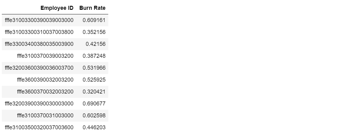
Combine the prediction with the test dataset. Then we can view the Burn Rate prediction of each EmployeeId.
df = test.cbind(preds)
df.head(2)

Slice columns by a vector of names to keep only the relevant columns in the final dataframe.
res = df[:, ["Employee ID", "predict"]]
res.head(2)

Rename the ‘predict’ column to ‘Burn Rate’.
res.set_names(['Employee ID','Burn Rate'])
Save Results
Save the results in a .CSV file.
h2o.export_file(res, path = "C:\Burnout_Rate_Prediction\dataset\submission.csv", force = True)

Save Leader Model
There are two ways to save the leader model — binary format and MOJO format. If you’re taking your leader model to production, then it’s suggested MOJO format since it’s optimized for production use.
h2o.save_model(aml.leader, path = "C:\Burnout_Rate_Prediction\h20_model")

aml.leader.download_mojo(path = "C:\Burnout_Rate_Prediction")

Ensemble Exploration
To understand how the ensemble works, let’s take a peek inside the Stacked Ensemble “All Models” model. The “All Models” ensemble is an ensemble of all of the individual models in the AutoML run. This is often the top-performing model on the leaderboard.
# Get model ids for all models in the AutoML Leaderboard
model_ids = list(aml.leaderboard['model_id'].as_data_frame().iloc[:,0])
# Get the "All Models" Stacked Ensemble model
se = h2o.get_model([mid for mid in model_ids if "StackedEnsemble_AllModels" in mid][0])
# Get the Stacked Ensemble metalearner model
metalearner = h2o.get_model(se.metalearner()['name'])
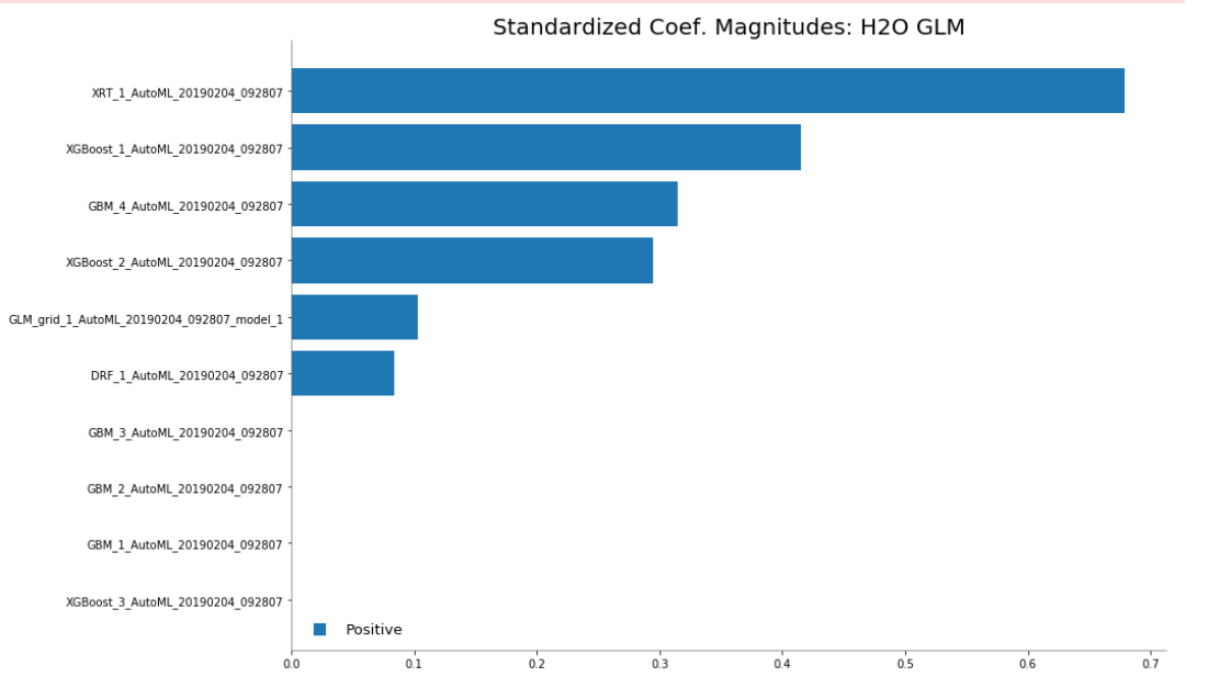
Examine the variable importance of the metalearner (combiner) algorithm in the ensemble. This shows us how much each base learner is contributing to the ensemble. The AutoML Stacked Ensembles use the default metalearner algorithm (GLM with non-negative weights), so the variable importance of the metalearner is actually the standardized coefficient magnitudes of the GLM.
metalearner.coef_norm()

We can also plot the base learner contributions to the ensemble.
Conclusion
H2O models can generate predictions in sub-millisecond scoring times. H2O AutoML offers APIs in several languages (R, Python, Java, Scala) which means it can be used seamlessly within a diverse team of data scientists and engineers. It is also available via a point-and-click H2O web GUI called Flow, which further reduces the barriers to the widespread use of automatic machine learning. Though the algorithm is fully automated, many of the settings are exposed as parameters to the user, so that certain aspects of the modeling steps can be customized. H2O also has tight integrations to big data computing platforms such as Hadoop and Spark and has been successfully deployed on supercomputers in a variety of HPC environments.
H2O has a very active and engaged user base in the open-source machine learning community. Key aspects of H2O AutoML include its ability to handle missing or categorical data natively, it’s comprehensive modeling strategy, including powerful stacked ensembles, and the ease in which H2O models can be deployed and used in enterprise production environments. The leaderboard features informative and actionable information such as model performance, training time, and per-row prediction speed for each model trained in the AutoML run ranked according to user preference.


