Introduction
The first step of any data-related process is the collection of data. Once we have collected the data, what do we do with it? Data can be sorted, analyzed, and used in various methods and formats, depending on the project’s needs. While analyzing a dataset, We use statistical methods to arrive at a conclusion. Data-driven decision-making also depends on how efficiently we use these methods. Two types of statistical methods are widely used in data analysis: descriptive and inferential. This article will focus more on descriptive statistics, its types, calculations, examples, etc.
This article was published as a part of the Data Science Blogathon.
Table of contents
- Types of Statistics
- What is Descriptive Statistics?
- What is Inferential Statistics?
- Types of Descriptive Statistics
- Descriptive Statistics Based on the Central Tendency of Data
- Descriptive Statistics Based on the Dispersion of Data
- Descriptive Statistics Based on the Shape of the Data
- Univariate Data vs. Bivariate Data in Descriptive Statistics
- Conclusion
- Frequently Asked Questions
Types of Statistics
When you delve into the world of statistics, you’ll encounter two fundamental branches: descriptive statistics and inferential statistics. These two distinct approaches help us make sense of data and draw conclusions. Let’s look at the differences between these two branches to shed light on their roles in the realm of statistical analysis.
| Aspect | Descriptive Statistics | Inferential Statistics |
|---|---|---|
| Purpose | Summarize and describe data | Draw conclusions or predictions |
| Data Sample | Analyzes the entire dataset | Analyzes a sample of the data |
| Examples | Mean, Median, Range, Variance | Hypothesis testing, Regression |
| Scope | Focuses on data characteristics | Makes inferences about populations |
| Goal | Provides insights and simplifies data | Generalizes findings to a larger population |
| Assumptions | No assumptions about populations | Requires assumptions about populations |
| Common Use Cases | Data visualization, data exploration | Scientific research, hypothesis testing |
What is Descriptive Statistics?
Descriptive statistics serves as the initial step in understanding and summarizing data. It involves organizing, visualizing, and summarizing raw data to create a coherent picture. The primary goal of descriptive statistics is to provide a clear and concise overview of the data’s main features. This helps us identify patterns, trends, and characteristics within the data set without making broader inferences.
Key Aspects of Descriptive Statistics
- Measures of Central Tendency: Descriptive statistics include calculating the mean, median, and mode, which offer insights into the center of the data distribution.
- Measures of Dispersion: Variance, standard deviation, and range help us understand the spread or variability of the data.
- Visualizations: Creating graphs, histograms, bar charts, and pie charts visually represent the data’s distribution and characteristics.
What is Inferential Statistics?
Inferential statistics takes data analysis to the next level by drawing conclusions about populations based on a sample. It involves making predictions, generalizations, and hypotheses about a larger group using a smaller subset of data. Inferential statistics bridges the gap between our data and the conclusions we want to reach. This is particularly useful when obtaining data from an entire population is impractical or impossible.
Key Aspects of Inferential Statistics
- Sampling Techniques: Inferential statistics relies on carefully selecting representative samples from a population to make valid inferences.
- Hypothesis Testing: This process involves setting up hypotheses about population characteristics and using sample data to determine if these hypotheses are statistically significant.
- Confidence Intervals: These provide a range of values within which we’re confident a population parameter lies based on sample data.
- Regression Analysis: Inferential statistics also encompass techniques like regression analysis to model relationships between variables and predict outcomes.
Now we will look at descriptive statistics in detail.
Types of Descriptive Statistics
There are various dimensions in which this data can be described. The three main dimensions used for describing data are the central tendency, dispersion, and the shape of the data. Now, let’s look at them in detail, one by one.
Descriptive Statistics Based on the Central Tendency of Data
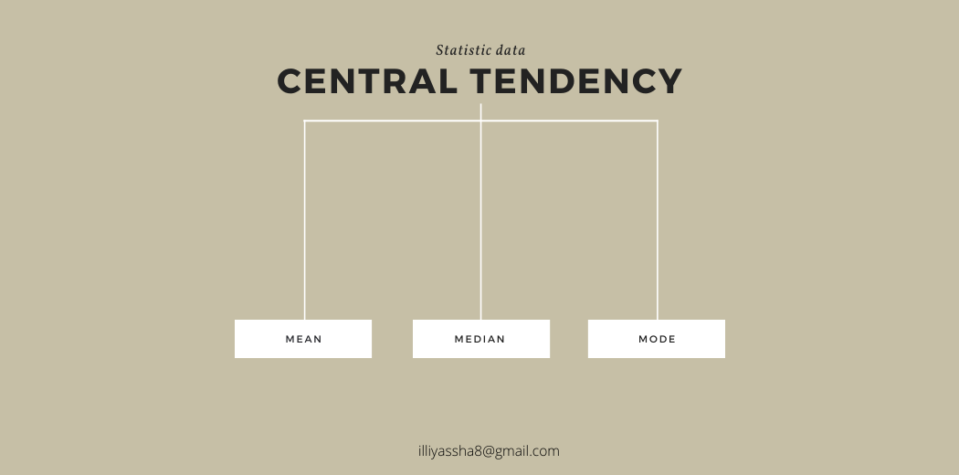
The central tendency of data is the center of the distribution of data. It describes the location of data and concentrates on where the data is located. The three most widely used measures of the “center” of the data are Mean, Median, and Mode.
Mean
The “Mean” is the average of the data. The average can be identified by summing up all the numbers and then dividing them by the number of observations.
Mean = X1 + X2 + X3 +… + Xn / n
Example:
Data – 10,20,30,40,50 and Number of observations = 5
Mean = [ 10+20+30+40+50 ] / 5
Mean = 30
The central tendency of the data may be influenced by outliers. You may now ask, ‘What are outliers?‘ Well, outliers are extreme behaviors. An outlier is a data point that differs significantly from other observations. It can cause serious problems in analysis.

Example:
Data – 10,20,30,40,200
Mean = [ 10+20+30+40+200 ] / 5
Mean = 60
Solution for the outliers problem: Removing the outliers while taking averages will give us better results.
Median
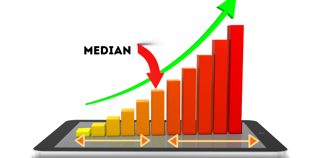
It is the 50th percentile of the data. In other words, it is exactly the center point of the data. The median can be identified by ordering the data, splitting it into two equal parts, and then finding the number in the middle. It is the best way to find the center of the data.
Note that, in this case, the central tendency of the data is not affected by outliers.
Example:
Odd number of Data – 10,20,30,40,50
Median is 30.
Even the number of data – 10,20,30,40,50,60
Find the middle 2 data and take the mean of those two values.
Here, 30 and 40 are middle values.
Now, add them and divide the result by 2
30+40 / 2 =35
Median is 35
Mode
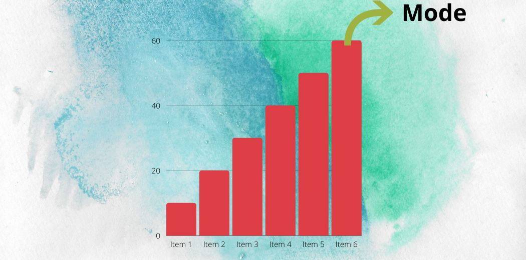
The mode of the data is the most frequently occurring data or elements in a dataset. If an element occurs the highest number of times, it is the mode of that data. If no number in the data is repeated, then that data has no mode. There can be more than one mode in a dataset if two values have the same frequency, which is also the highest frequency.
Outliers don’t influence the data in this case. The mode can be calculated for both quantitative and qualitative data.
Example:
Data – 1,3,4,6,7,3,3,5,10, 3
Mode is 3, because 3 has the highest frequency (4 times)
Descriptive Statistics Based on the Dispersion of Data
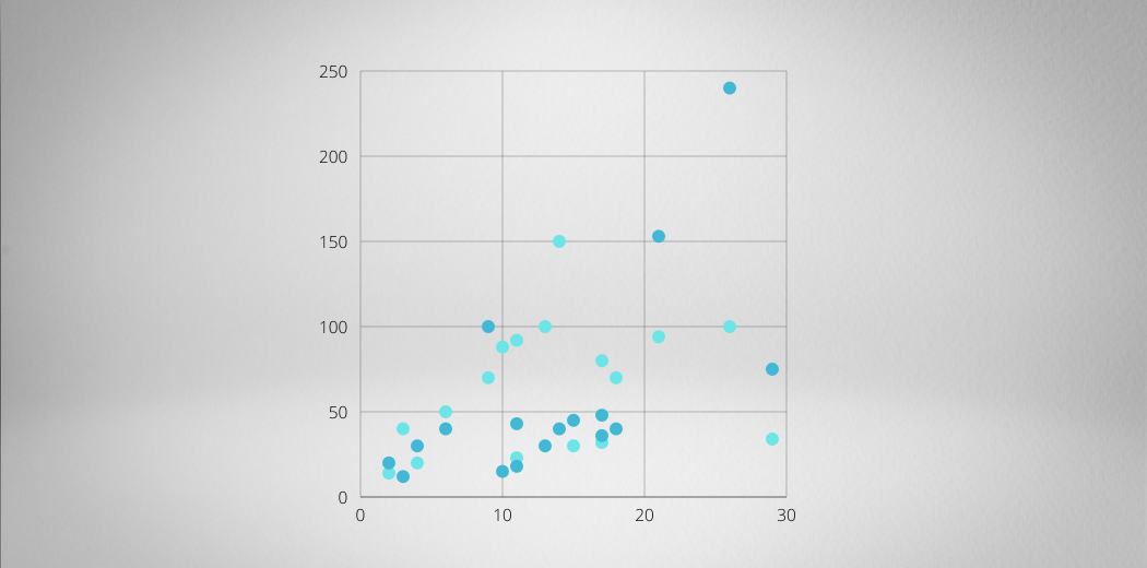
The dispersion is the “spread of the data”. It measures how far the data is spread. In most of the dataset, the data values are closely located near the mean. The values are widely spread out of the mean on some other datasets. These dispersions of data can be measured by the Inter Quartile Range (IQR), range, standard deviation, and variance of the data.
Let us see these measures in detail.
Inter Quartile Range (IQR)
Quartiles are special percentiles.
1st Quartile Q1 is the same as the 25th percentile.
2nd Quartile Q2 is the same as 50th percentile.
3rd Quratile Q3 is same as 75th percentile
Steps to find quartile and percentile
- The data should sorted and ordered from the smallest to the largest.
- For Quartiles, ordered data is divided into 4 equal parts.
- For Percentiles, ordered data is divided into 100 equal parts.
The Inter Quartile Range is the difference between the third quartile (Q3) and the first quartile (Q1)
IQR = Q3 – Q1
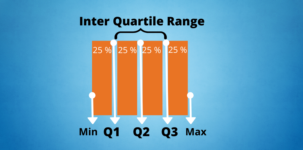
In this example, the Inter Quartile range is the spread of the middle half (50%) of the data.
Range
The range is the difference between the largest and the smallest value in the data.
Standard Deviation
The most common measure of spread is the standard deviation. The Standard deviation measures how far the data deviates from the mean value. The standard deviation formula varies for population and sample. Both formulas are similar but not the same.
- Symbol used for Sample Standard Deviation – “s” (lowercase)
- Symbol used for Population Standard Deviation – “σ” (sigma, lower case)
Steps to find the Standard Deviation
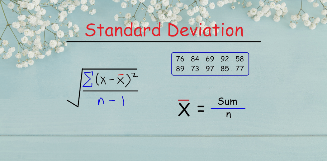
If x is a number, then the difference “x – mean” is its deviation. The deviations are used to calculate the standard deviation.
Sample Standard Deviation, s = Square root of sample variance
Sample Standard Deviation, s = Square root of [Σ(x − x ¯ )2/ n-1] where x ¯ is average and n is no. of samples
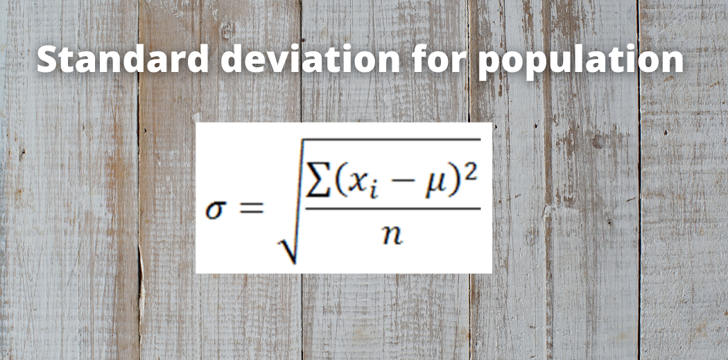
Population Standard Deviation, σ = Square root of population variance
Population Standard Deviation, σ = Square root of [ Σ(x − μ)2 / N ] where μ is Mean and N is no.of population.
The standard deviation is always positive or zero. It will be large when the data values are spread out from the mean.
Variance
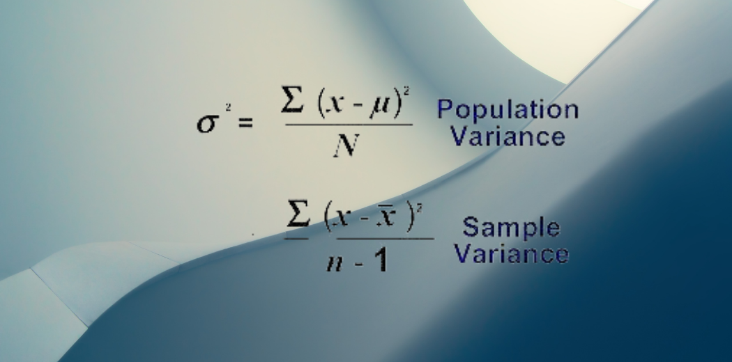
The variance is a measure of variability. It is the average squared deviation from the mean. The symbol σ2 represents the population variance, and the symbol for s2 represents sample variance.
Population variance σ2 = [ Σ(x − μ)2 / N ]Sample Variance s2 = [ Σ(x − x ¯ )2/ n-1 ]
Descriptive Statistics Based on the Shape of the Data
The shape of the data is important because deciding the probability of data is based on its shape. The shape describes the type of the graph.
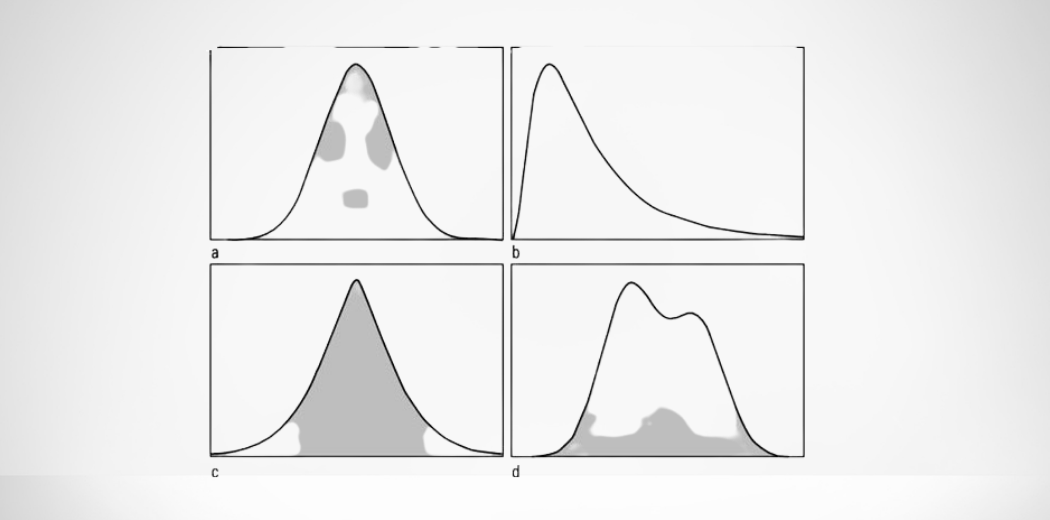
The shape of the data can be measured by three methodologies: symmetric, skewness, kurtosis
Symmetric
In the symmetric shape of the graph, the data is distributed the same on both sides. In symmetric data, the mean and median are located close together. The curve formed by this symmetric graph is called a normal curve.
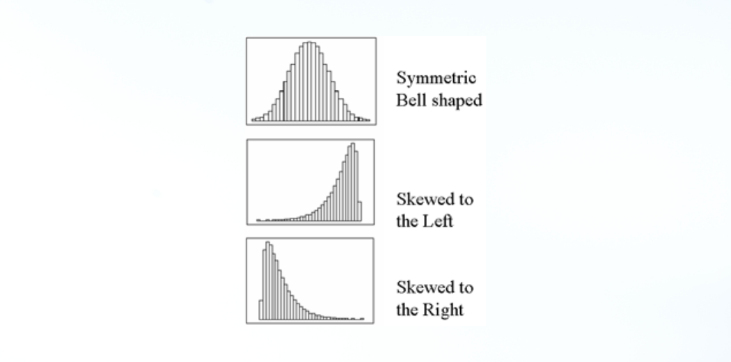
Skewness
Skewness is the measure of the asymmetry of the distribution of data. The data is not symmetrical (i.e.) it is skewed towards one side. Skewness is classified into two types: positive skew and negative skew.
- Positively skewed: In a Positively skewed distribution, the data values are clustered around the left side of the distribution, and the right side is longer. The mean and median will be greater than the mode in the positive skew.
- Negatively skewed: In a Negatively skewed distribution, the data values are clustered around the right side of the distribution, and the left side is longer. The mean and median will be less than the mode.
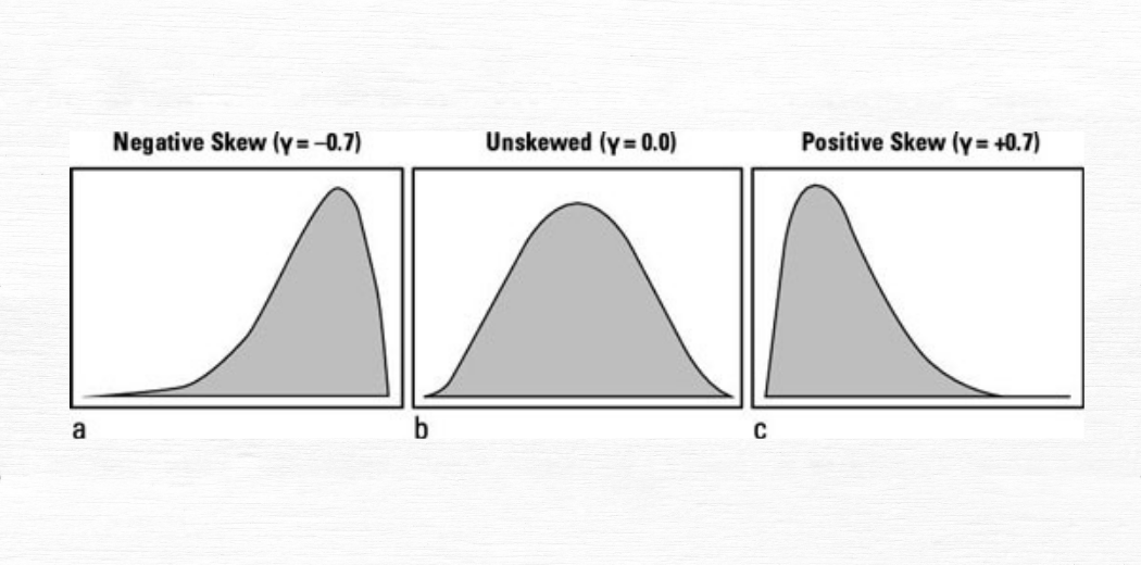
Kurtosis
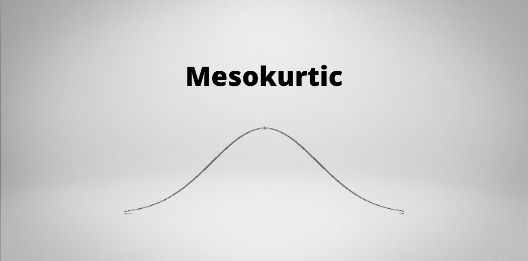
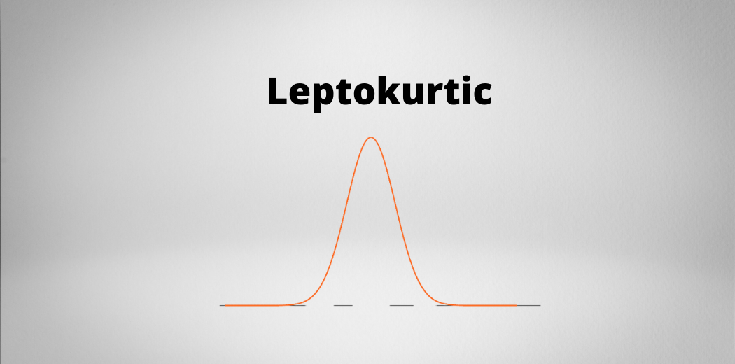
Kurtosis is the measure of describing the distribution of data. This data is distributed in three different ways: platykurtic, mesokurtic, and leptokurtic.
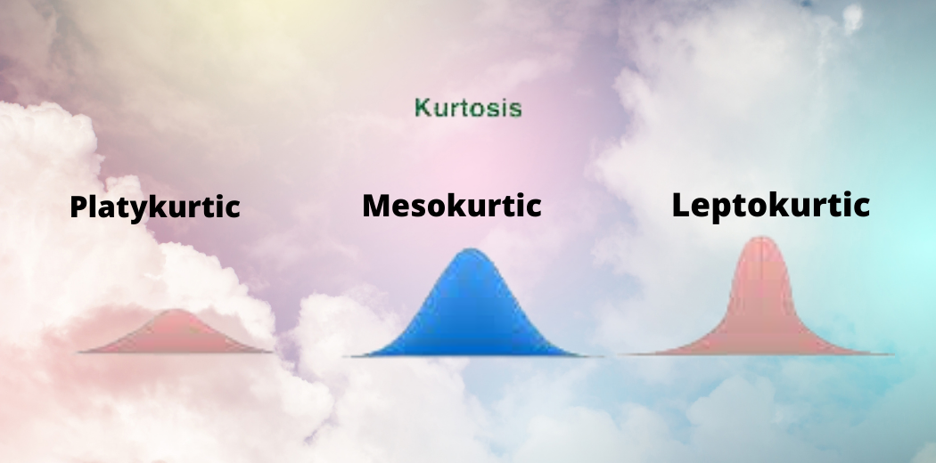
- Platykurtic: The platykurtic shows a distribution with flat tails. Here, the data is distributed fairly. The flat tails indicated the small outliers in the distribution.

- Mesokurtic: In Mesokurtic, the data is widely distributed. It is normally distributed, and it also matches normal distribution.
- Leptokurtic: In leptokurtic, the data is very closely distributed. The height of the peak is greater than the width of the peak.
Univariate Data vs. Bivariate Data in Descriptive Statistics
When it comes to delving into the world of data analysis, two key terms you’re likely to encounter are “univariate” and “bivariate.” These terms are crucial in descriptive statistics, as they help us categorize and understand the data types we’re working with. Whether you’re deciphering the properties of individual data points or unraveling the intricate dance between two variables, the concepts of univariate and bivariate data provide the foundation for insightful data analysis.
the key difference between univariate and bivariate data lies in the focus of analysis. Univariate analysis centers on understanding the characteristics of a single variable, while bivariate analysis explores connections and interactions between two variables. Let’s break down the differences between univariate and bivariate data to better grasp their significance.
Univariate Data
Univariate data focuses on a single variable, essentially spotlighting one aspect of your data. In this scenario, you’re interested in studying the distribution, central tendency, and dispersion of a single set of values. For instance, if you’re analyzing the heights of a group of individuals, you’re dealing with univariate data. Here, the variable of interest is height, and you aim to uncover insights about that specific characteristic.
In univariate analysis, you’re often looking at measures like:
- Measures of Central Tendency: Mean, median, and mode provide insights into where the center of the data lies.
- Measures of Dispersion: Range, variance, and standard deviation help you understand how spread out the data is.
- Frequency Distribution: Creating histograms, bar charts, and pie charts allows you to visualize the data’s distribution.
Bivariate Data
Bivariate data, on the other hand, adds an extra layer of complexity to your analysis by involving two variables. Here, you’re not just interested in understanding individual characteristics; you’re also keen on uncovering relationships and patterns between two different variables. For example, if you’re examining the relationship between hours of study and exam scores, you’re working with bivariate data. The goal is to determine whether changes in one variable (study hours) have an impact on another (exam scores).
Bivariate analysis often involves techniques such as:
- Scatter Plots: These visualizations showcase the relationship between two variables, with each data point plotted on the graph.
- Correlation: Calculating correlation coefficients helps you quantify the strength and direction of the relationship between variables.
- Regression Analysis: This technique allows you to model the relationship between variables, predicting the outcome of one based on the other.
Conclusion
In a world flooded with data, understanding, interpreting, and communicating information is paramount. Descriptive statistics doesn’t just crunch numbers; it crafts narratives, constructs visualizations, and empowers us to make informed decisions. Hope this article has given you a brief introduction to descriptive statistics. In this article, we have seen how the various measures of descriptive statistics, such as central tendency, dispersion, and shape of the data curve, help decipher the numbers. We have also bridged the gap between individual characteristics and the dance between variables by learning about univariate and bivariate data.
Frequently Asked Questions
Ans. The methods used to summarize and describe the main features of a dataset are called descriptive statistics. Measures of central tendencies, measures of variability, etc., which give information about the typical values in a dataset, are all examples of descriptive statistics.
Ans. The 5 descriptive statistics include standard deviation, minimum and maximum variables, variance, kurtosis, and skewness.
Ans. The frequency distribution, central tendency, and variability of a dataset are the 3 main types of descriptive statistics.
Ans. Descriptive statistics are of 3 types: frequency distribution, central tendency, and variability.
The media shown in this article are not owned by Analytics Vidhya and are used at the Author’s discretion.


