What are Anomalies and to detect them? What impact it has on the data?
Introduction
Anomalies are the points different from the normal state of existence. These are something that can arise due to different circumstances based on the several factors impacting it. For example, the tumors that are developed due to some diseases like when a person is diagnosed with cancer then more number of cells developed without any limit.
In the same way, when we get such data we must analyze and detect these anomalies so that it becomes easier for treatment and knowing what actions to be taken. When such anomalies occur in the automobile industry like when the sales of a particular car or other transport vehicles are high or low. Then it is an anomaly out of the whole data. Anomalies are nothing other than the outliers in the data.
How do you detect the outliers or What are the methods used for detecting anomalies?
1. Using data visualization(like making use of boxplots, violin plots…etc)
2. Using Statistical methods like Quantile methods(IQR, Q1, Q3), Finding Minimum, Maximum, and median of the data, Z-score, etc.
3. ML algorithms like IsolationForest, LocalOutlierFactor, OneClassSVM, Elliptic Envelope …etc.
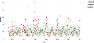
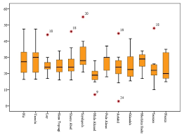
1. Data Visualization: When a feature a plotted using visualization tools like seaborn, matplotlib, plotly, or other software like tableau, PowerBI, Qlik Sense, Excel, Word, …etc we get an idea of the data and its count in the data also we get to know the anomalies mainly using boxplots, violin plots, scatter plots.
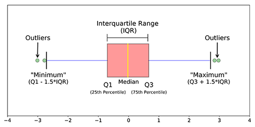
2. Statistical methods: When you find the mean of the data it may not give the correct middle value when anomalies are present in the data. When anomalies exist in the data median gives a correct value than the mean because the median sorts the values and finds the middle position in the data whereas the mean just averages the values in the data. To find the outliers in the right and left side of the data you use Q3+1.5(IQR), Q1-1.5(IQR). Also by finding the maximum, minimum, and median of the data you can say whether the anomalies are present in the data or not.
3. ML algorithms: The benefit of using the unsupervised algorithms for anomaly detection is we can find anomalies for multiple variables or features or predictors in the data at the same times instead of separately for individual variables. It can also be done both ways called Univariate Anomaly detection and Multivariate Anomaly detection.
a. Isolation Forest: This is an unsupervised technique of detecting anomalies when labels or true values are not present. It would be a complex task for checking each row in the data for detecting such rows which can be considered as anomalies.
Isolation Forest is a tree-based model. The trees formed for this is not the same as it is done in the decision trees. Decision trees and Isolation Forests are different ways of construction. Also, one more main difference is Decision tree is a supervised learning algorithm and the Isolation Forest is an Unsupervised learning algorithm.
In these Isolation trees, partitions are created by first randomly selecting a feature or variable then selecting a random split value between the minimum and maximum value of the selected feature. Again, the root node is selected randomly without any condition for being a root node like it happens in the decision tree. The root node is selected randomly from the variables in the data then some random value is taken which is in between the maximum and minimum of that particular feature.
The anomaly score of an input sample is computed as the mean anomaly score of the trees in the Isolation forest. Then the anomaly score is calculated for each variable after fitting the entire data to the model. When the anomaly score soars up there is a high chance that it is an anomaly than the row which has less anomaly score. There are three functions in this algorithm which is making it simple for seeing and storing the scores easily using the few lines of code which is given below:
from sklearn.ensemble import IsolationForest
isolation_forest = IsolationForest(n_estimators=1000, contamination=0.08)
isolation_forest.fit(df['Rate'].values.reshape(-1, 1))
df['anomaly_score_rate'] = isolation_forest.decision_function(df['rate'].values.reshape(-1, 1))
df['outlier_univariate_rate'] = isolation_forest.predict(df['rate'].values.reshape(-1, 1))
Here contamination parameter plays a major role in detecting more anomalies. Contamination is the percentage of values you are giving to the algorithm that there is this much percentage of anomalies in the data. Eg: When you gave 0.10 as contamination value then algorithms consider that there are 10% of anomalies in the data. By finding the optimal contamination you would be able to detect anomalies with a good number.
When you want to do Multivariate anomaly detection you have to first normalize the values in the data so that algorithm can give correct predictions. Normalization or Standardization is essential when dealing with continuous values.
minmax = MinMaxScaler(feature_range=(0, 1))
X = minmax.fit_transform(df[['rate','scores']])
clf = IsolationForest(n_estimators=100, contamination=0.01, random_state=0)
clf.fit(X)
df['multivariate_anomaly_score'] = clf.decision_function(X)
df['multivariate_outlier'] = clf.predict(X)
For knowing more go to sklearn Isolation Forest
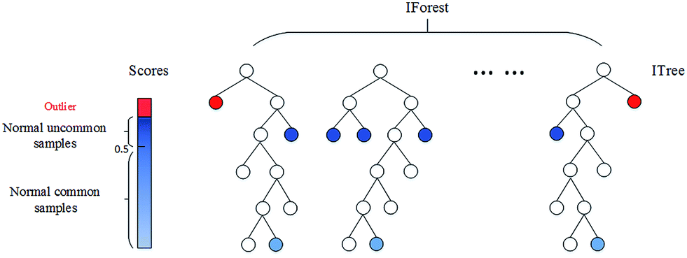
The above image credits to – https://pubs.rsc.org/en/content/articlelanding/2016/ay/c6ay01574c#!divAbstract
b. LocalOutlierFactor: This is also an unsupervised algorithm and it is not tree-based than a density-based algorithm like KNN, Kmeans. When any data point is taken into account as an outlier depending upon its local neighborhood, it’s a local outlier. LOF will identify an outlier considering the density of the neighbor. LOF performs well when the density of the data point isn’t constant throughout the dataset.
There are two types of detection made using this algorithm. They are outlier detection and novelty detection where outlier detection is unsupervised and novelty detection is semi-supervised as it uses the train data for making its predictions on test data even though train data doesn’t contain exact predictions.
Even LocalOutlierFactor uses the same code then the code is used only for novelty detection when the novelty parameter is True in this model. When its default False then outlier detection would be used where the only fit_predict would work. When novelty=True this function is disabled.
Below is the code for finding anomalies using the Local Outlier Factor algorithm
minmax = MinMaxScaler(feature_range=(0, 1))
X = minmax.fit_transform(df[['rate','scores']])
# Novelty detection
clf = LocalOutlierFactor(n_neighbors=100, contamination=0.01,novelty=True) #when novelty = True
clf.fit(X_train)
df['multivariate_anomaly_score'] = clf.decision_function(X_test)
df['multivariate_outlier'] = clf.predict(X_test)
# Outlier detection
local_outlier_factor_multi=LocalOutlierFactor(n_neighbors=15,contamination=0.20,n_jobs=-1) # when novelty = False
multi_pred=local_outlier_factor_multi.fit_predict(X)
df1['Multivariate_pred']=multi_pred
For knowing more about this refer sklearn Local Outlier Factor
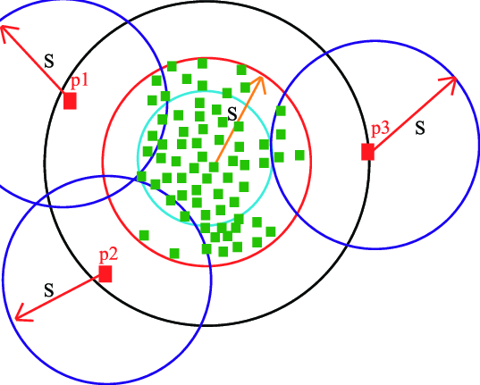
c. One-class SVM: There is Supervised SVM which deals with regression and classification tasks. Here is an unsupervised One-class SVM as the labels are unknown. One-class SVMs are a special type of support vector machine. First, data is modeled and the algorithm is trained. Then when new data are encountered their position relative to the normal data (or inliers) from training can be used to determine whether it is out of class or not. As they can be trained with unlabelled data or without target variables in it they are an example of unsupervised machine learning.
It has just a few lines of code as other algorithms:
from sklearn.svm import OneClassSVM
pred=clf.predict(X)
anomaly_score=clf.score_samples(X)
clf = OneClassSVM(gamma='auto',nu=0.04,gamma=0.0004).fit(X)
To know more refer to this site of sklearn for One-class SVM
d. Elliptic Envelope Algorithm: This algorithm is used when the data is Gaussian distributed. In this it is like this model converts the data into elliptical shape and the points which are far away from this shape coordinates are considered outliers and for this minimum-covariance- determinant is found out. It is like when finding the covariance in the dataset so that minimum is excluded and which is higher those points are considered anomalies. The below picture depicts the explanation for this algorithm detection.
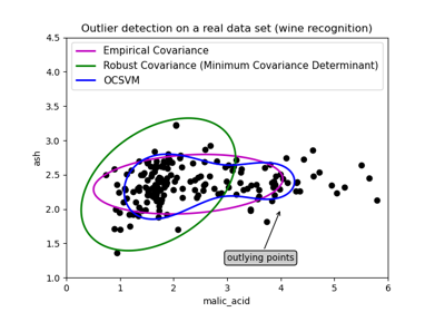
It has the same line of code as just to fit the data and predict on the same which identifies the anomalies in the data where -1 is allotted for anomalies and +1 for normal data or in-liers.
from sklearn.covariance import EllipticEnvelope
model1 = EllipticEnvelope(contamination = 0.1) # fit model
model1.fit(X_train)
model1.predict(X_test)
For knowing more about parameters and comparison chart refer to sklearn Elliptic Envelope
These are some of the techniques used in anomaly detection which helps in knowing the points which are far away from the normal and bringing a lot of unexpected changes in the data. Based on the place or type of data it has various effects and used in many places and industries like the medical industry, automobile industry, construction industry, food industry( anomalies which are different from prescribed standards), defense industry…etc.
Let me know if you have any queries. Thanks for reading.👩🕵️♀️👩🎓 Have a nice day.😊
The media shown in this article are not owned by Analytics Vidhya and is used at the Author’s discretion.


