This article was published as a part of the Data Science Blogathon.
Introduction
Have you ever thought about how machines can tell whether a person has a disease or not by just analyzing their images? Have you heard of a recent revolutionary invention of FastTag, which significantly reduces the waiting time of vehicles in tool booths, or have you ever wondered how the face recognition system of your smartphone works? All these are examples of Image Classification.
In layman’s terms, categorizing and identifying sets of pixels or vectors inside an image by predetermined criteria is known as image classification. It is possible to develop the classification legislation using one or more spectral or textural properties. “Supervised” and “unsupervised” categorization techniques are two common types.
In this article, we will learn how we can create neural network models to perform classification on IRIS Dataset. We will also tune the accuracy by tuning these many parameters like Vary learning rate, Varying the number of epochs, Random weight initialization, Using SGD optimizer, Using activation functions: sigmoid, tanh.
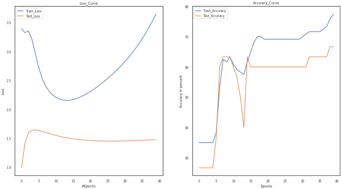
Use cross-entropy loss. We will also plot the loss and accuracy curves on the training and test sets. To support our claim, we will find the best configuration for our network (a combination of the best learning rate, the best number of epochs, and the activation function).
What is Hyperparameter Tuning
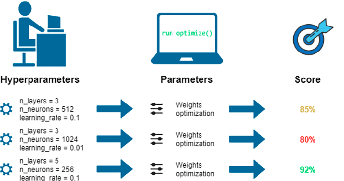
The number of neurons, activation function, optimizer, learning rate, batch size, and epochs are the hyperparameters that need to be tuned. We must adjust the number of layers must be in the second stage. Other traditional algorithms do not possess this.
Finding a set of ideal hyperparameter values for a learning algorithm and using this tuned algorithm on any data set is hyperparameter tuning. The model’s performance is maximized using that set of hyperparameters, which minimizes a predetermined loss function and results in better outcomes with fewer mistakes.
Some insights about the dataset:
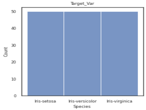
1. It consists of three classes: Setosa, Versicolor, and Virginia.
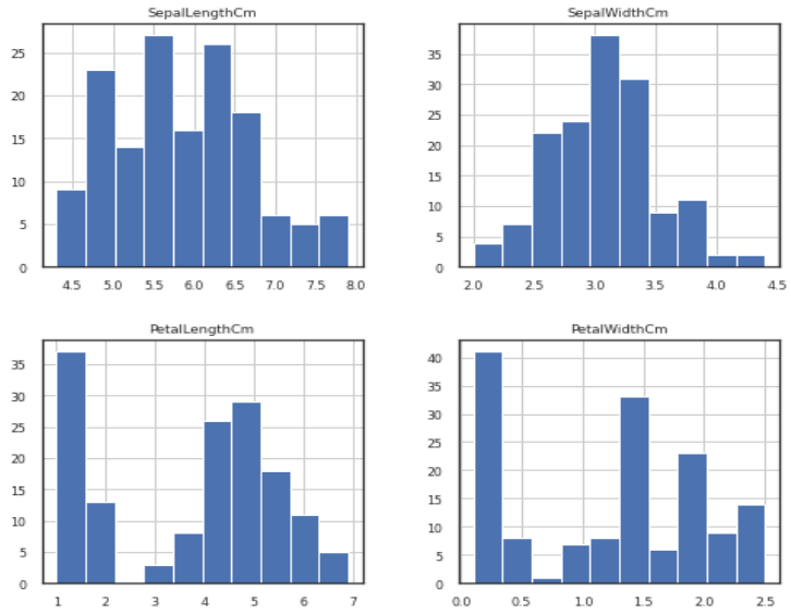
2. There are four different features: sepal length, sepal width, petal length, and petal width.
3. You can download the complete dataset from this link.
Code Implementation
1. Importing Libraries:
Below are all the required libraries during the execution of the code. Some are math, which is used to perform mathematical functions. Like pandas used in loading and pre-processing of the dataset, etc.
import math
import random
import numpy as np
from math import exp
import pandas
from them.autonotebook import tqdm
from matplotlib import pyplot as plt
import matplotlib as mlt
import seaborn
from random import seed
from random import random
2. Loading Dataset:
We will load the downloaded CSV file using Pandas library
3. Pre-processing of Dataset: Python Code:
We will drop the column of Id as we don’t require this field in this article. After that, we will use a label encoder to convert all the categorical data to numerical data. Finally, we will divide our dataset into the training and testing sets using sklearn’s train_test_split method.
df = df.drop('Id',axis=1)
epc, iter, arg1, ret, var2 = 0, 1, 1e-2, 1e-3, 1e-5
n_epoch1, n_epoch2, n_epoch3 = 15, 20, 25
If = df.drop(['Species'], axis=1)
If
Df = df['Species']
Df
Df = sklearn.preprocessing.LabelEncoder().fit_transform(Df)
Df
import sklearn
tests_size = 0.20
trains_size = 0.80
var = True
x_train, x_test, y_train, y_test = sklearn.model_selection.train_test_split(If, Df, test_size = tests_size, shuffle = var)
value_train = x_train.values
value_test = x_test.values
x_train = value_train
x_test = value_test
Loss Function:
The loss function assesses how your machine learning algorithm predicts the featured data set. In other words, loss functions gauge how well your model can forecast the desired result.
Optimal SGD:
The SGD method expands on the Gradient Descent and fixes various issues with the GD algorithm. The drawback of gradient descent is that it uses a lot of memory to load the complete n-point dataset at once to compute the derivative of the loss function.
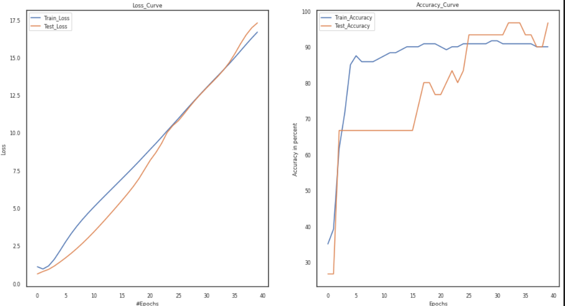
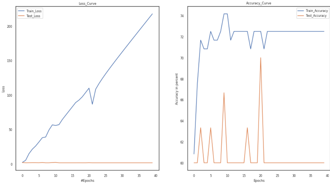
Vary the Learning Rate:
The “learning rate” or “step size” refers to how frequently the weights are changed during training. In particular, the learning rate is a hyperparameter that can be customized and used to train neural networks. Its value is typically modest and positive, falling between 0.0 and 1.0.
We will vary the learning rate from 0.001 to 0.002 to 0.003 and observe the changes.
lr_value = [1e-3, 1e-2, 1e-1]
model = Training_Model()
channel, tere = 3, 0
activation1, activation2 = 'tanh', 'sigmoid'
s1 = Add_layers(channel, activation=activation1)
s2 = Add_layers(channel, activation=activation2)
model.joinl(s1)
model.joinl(s2)
config.lr = lr_value[tere]
p1,p2,p3, p4 = loss,train_loader, test_loader, optimizer
model.configr(config, loss_function = p1, optimizer= p4, train_loader = p2,test_loader = p3)
history = model.fit()
plot(history)
Vary Number of Layers:
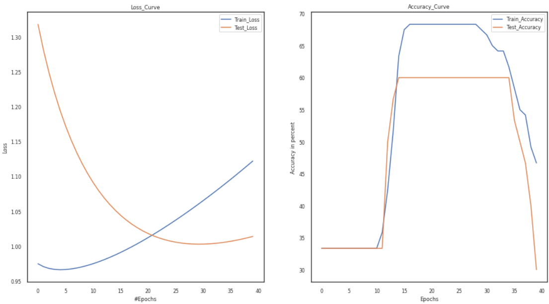
Convolution, pooling, normalizing, and many other layers are examples. For instance, MaxPool is significant since it reduces sensitivity to the position of features. We’ll go through each layer and examine its importance as we go.
In the code below, we will change the number of layers, keep everything the same, and then observe the change in loss and accuracy curves.
model = Training_Model()
channel, fg =3,0.001
activation1, activation2 = 'sigmoid', 'sigmoid'
s1 = Add_layers(channel, activation=activation1)
s2 = Add_layers(channel, activation=activation2)
model.joinl(s1)
model.joinl(s2)
config.LR = fg
p1,p2,p3, p4 = loss,train_loader, test_loader, optimizer
model.configr(config, loss_function = p1, optimizer= p4, train_loader = p2,test_loader = p3)history = model.fit()
model_summary(model)
plot(history)
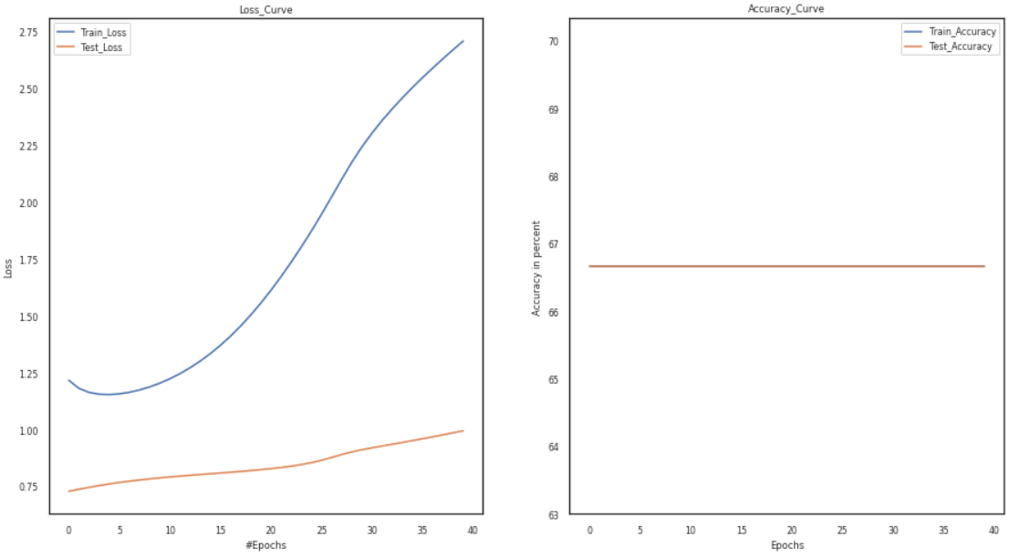
Vary Tanh and Relu Activation Functions:
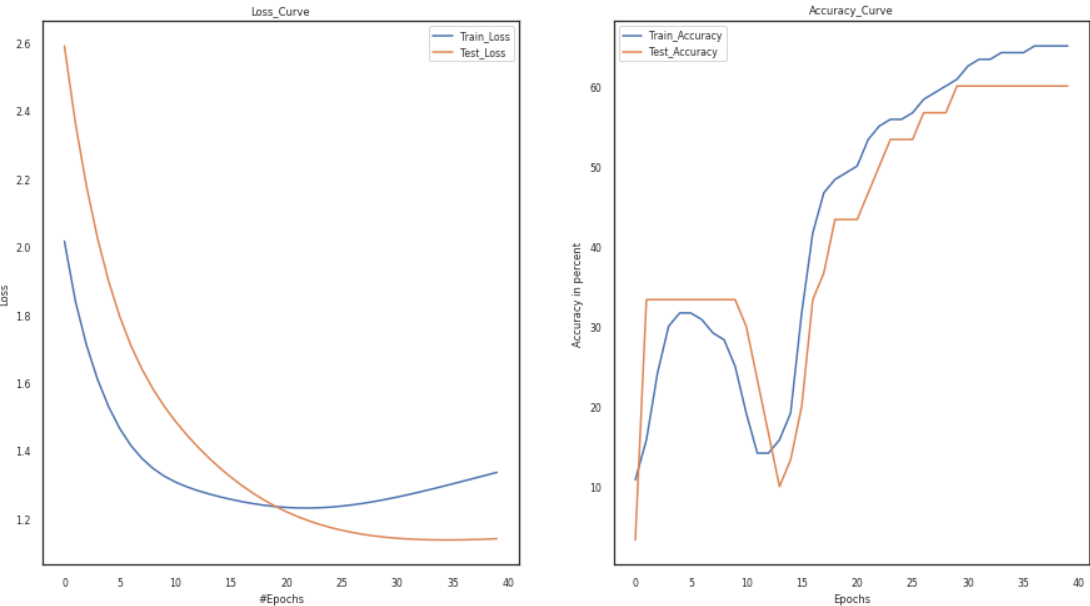
An artificial neural network may learn complicated patterns in the data with the aid of an activation function, which is a function that is introduced to the network. In contrast to a neuron-based model in human brains, the activation function determines what we should send signals to the next neuron at the end.
In the below code, we will change the activation function firstly as Relu and then Tanh and compare the accuracy and loss curves in both of them. We will add different layers containing different activation functions as per our needs.
model = Training_Model()
channel, temp1 = 3, 0.001
activation1, activation2 = 'relu', 'sigmoid'
s1 = Add_layers(channel, activation=activation1)
s2 = Add_layers(channel, activation=activation2)
model.joinl(s1)
model.joinl(s2)
config.LR = temp
p1,p2,p3, p4 = loss,train_loader, test_loader, optimizer
model.configr(config, loss_function = p1, optimizer= p4, train_loader = p2,test_loader = p3)
history = model.fit()
model_summary(model)
plot(history)
Vary Epochs:
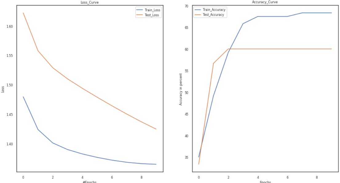
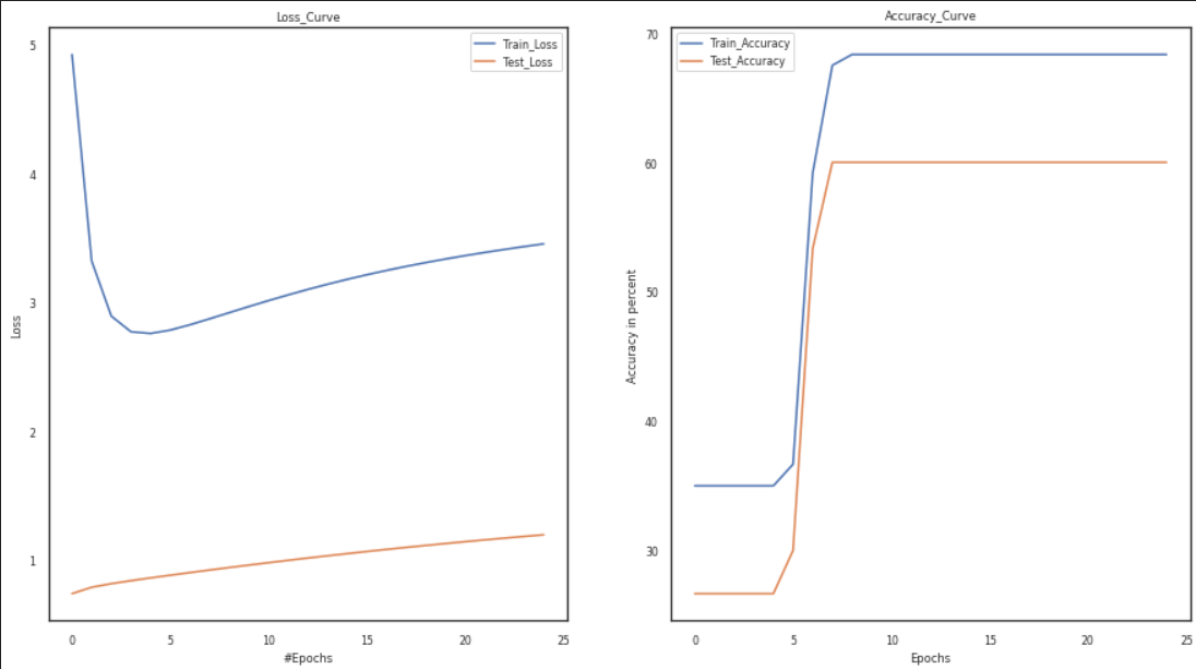
The word “epoch” is applied to the number of passes the machine learning algorithm has made across the training dataset. Typically, datasets are organized into batches (especially when the data is extensive).
In the code below, we will take the number of epochs first as five and then as 12, keep everything as it is, and then observe the loss and accuracy curves.
model = Training_Model()
channel, temp, temp1 =3, 0.001, 5
temp1 +=5
activation1, activation2 = 'tanh', 'sigmoid'
s1 = Add_layers(channel, activation=activation1)
s2 = Add_layers(channel, activation=activation2)
model.joinl(s1)
model.joinl(s2)
config.LR, config.epochs = temp, temp1
p1,p2,p3, p4 = loss,train_loader, test_loader, optimizer
model.configr(config, loss_function = p1, optimizer= p4, train_loader = p2,test_loader = p3)history = model.fit()
model_summary(model)
plot(history)
Results
As a result of the preceding experiments, we can conclude that the weight initialization approach significantly impacts the model’s accuracy. The vanishing gradient and overfitting problems develop due to erroneous weight initialization. As a result, the graphs show that better optimization and faster convergence are impossible. Furthermore, compared to other hyperparameter tuning methods, the combination of the tanh and sigmoid functions is an excellent choice for hyperparameters since it helps attain higher accuracy. Furthermore, the plots of the loss and accuracy curves show an improvement in accuracy with a decrease in the loss curves.
Furthermore, the use of sigmoid and tanh activations, as well as random weight initialization, can be solved by using the activation function of Relu or leaky relu, as well as better optimizers like Adam and better weight initialization approaches like He or Xavier initialization.
Conclusion
You can download the complete code of this article using this link.
In this article, we have learned how to train a convolutional neural network to train an IRIS Dataset. We will also check the performance of our model by varying various hyperparameters like Learning Rate, No. of epochs, Activation Function, and No. Of Layers.
In layman’s terms, optimization means programs or techniques that modify your neural network’s weights and learning rates to minimize losses. Optimizers facilitate quicker outcomes.
Despite the above hyperparameters, there are also many hyperparameters in the CNN model, like the size of kernels, number of kernels, length of strides, and pooling size, which directly affect the performance and training speed of CNNs.
An inbuilt library named Keras-tuner can automatically give you the best hyperparameters that suit your dataset and classification problem. We will discuss more in upcoming blogs.
Major points of this article:
1. Firstly, we have discussed the dataset, its code for loading and pre-processing also visualize it.
2. After that, we discussed the code for model training, in which we discussed code for the loss function, activation function, CNN layers, etc.
3. Further, we have discussed the various hyperparameters tuning like learning rate, no. of epochs, etc.
4. Finally, the article discusses the best set of hyperparameters that suits our model.
I hope you have enjoyed my article. Please like and share it and comment below if you have any doubts.
The media shown in this article is not owned by Analytics Vidhya and is used at the Author’s discretion.


