Beginner’s Guide To Logistic Regression Using Python

20 July 2024

1

This article was published as a part of the Data Science Blogathon.

Overview

What Is Logistic Regression
Mathematics Involved in Logistic Regression
Performance Measuring via Confusion Matrices
Demonstration of Logistic Regression with Python Code

Logistic Regression is one of the most popular Machine Learning Algorithms, used in the case of predicting various categorical datasets. Categorical Datasets have only two outcomes, either 0/1 or Yes/No

1. What Is Logistic Regression?

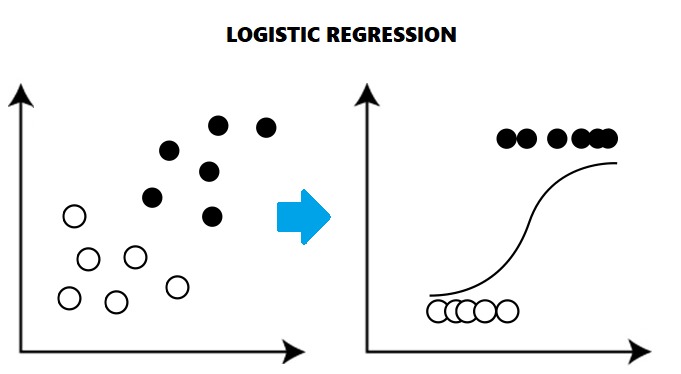
It is a type of Regression Machine Learning Algorithms being deployed to solve Classification Problems/categorical,

Problems having binary outcomes, such as Yes/No, 0/1, True/False, are the ones being called classification problems.

2. Why Apply Logistic Regression?

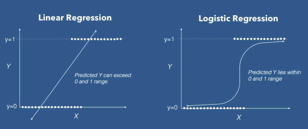
Linear regression doesn’t give a good fit line for the problems having only two values(being shown in the figure), It will give less accuracy while prediction because it will fail to cover the datasets, being linear in nature.

For the best fit of categorical datasets, a Curve is being required which is being possible with the help of Logistic Regression, as it uses a Sigmoid function to make predictions

3. Mathematics Involved in Logistic Regression

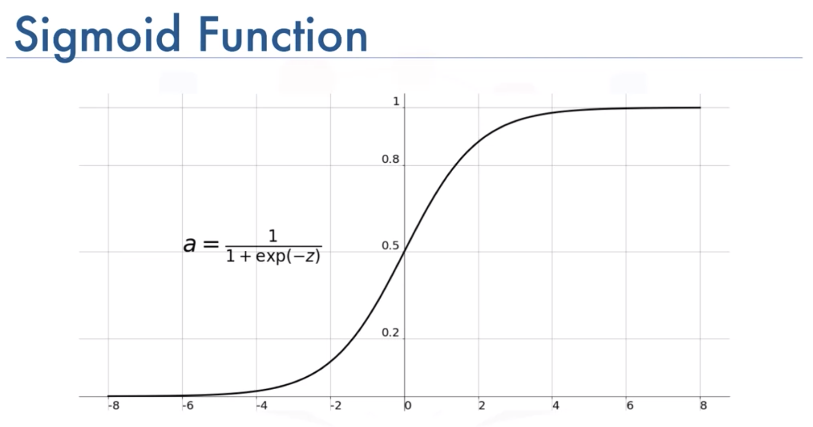
The main reason behind bending of the Logistic Regression curve is because of being calculated using a Sigmoid Function (also known as Logistic Function because being used in logistic regression) being given below

This the mathematical function which is having the ‘S – Shaped curve’. The value of the Sigmoid Function always lies between 0 and 1, which is why it’s being deployed to solve categorical problems having two possible values.

Mathematics Involved in Logistic Regression sigmoid

4. Implementation Of Logistic Regression In Making Predictions

Logistic Regression deploys the sigmoid function to make predictions in the case of Categorical values.

It sets a cut-off point value, which is mostly being set as 0.5, which, when being exceeded by the predicted output of the Logistic curve, gives respective predicted output in form of which category the dataset belongs

For Example,

In the case of the Diabetes prediction Model, if the output exceeds the cutoff point, prediction output will be given as Yes for Diabetes otherwise No, if the value is below the cutoff point

5. Measuring Performance

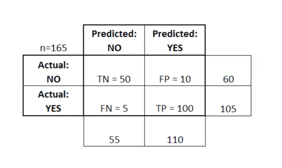
For measuring the performance of the model solving classification problems, the Confusion matrix is being used, below is the implementation of the Confusion Matrix.

Key terms:

– TN Stands for True Negatives(The predicted(negative) value matches the actual(negative) value)
– FP stands for False Positives (The actual value, was negative, but the model predicted a positive value)
– FN stands for False Negatives(The actual value, was positive, but the model predicted a negative value)
– TP stands for True Positives(The predicted(positive) value matched the actual value(positive))

For a good model, one should not have a high number of False Positive or False Negative

6. Key Features Of Logistic Regression

1. Logistic regression is one of the most popular Machine Learning algorithms, used in the Supervised Machine Learning technique. It is used for predicting the categorical dependent variable, using a given set of independent variables.

2. It predicts the output of a categorical variable, which is discrete in nature. It can be either Yes or No, 0 or 1, true or False, etc. but instead of giving the exact value as 0 and 1, it gives the output as the probability of the dataset which lies between 0 and 1.

3. It is similar to Linear Regression. The only difference is that Linear Regression is used for solving Regression problems, whereas Logistic regression is used for solving the classification problems/Categorical problems.

4 In Logistic regression, the “S” shaped logistic (sigmoid) function is being used as a fitting curve, which gives output lying between 0 and 1.

7. Types of Logistic Regression

There Are Three Types:

a Binomial

b Ordinal

c Multinomial

a Binomial

Binomial Logistic regression deals with those problems with target variables having only two possible values, 0 or 1.

Which can Signify Yes/No, True /False, Dead/Alive, and other categorical values.

b Ordinal

Ordinal Logistic Regression Deals with those problems whose target variables can have 3 or more than 3 values, unordered in nature. Those values don’t have any quantitative significance

For Example Type 1 House, Type 3 House, Type 3 House, etc

c Multinomial

Multinomial Logistic regression, just Ordinal Logistic Regression, deals with Problems having target values to be more than or equal to3. The main difference lies that unlike Ordinal, those values are well ordered. The values Hold Quantitative Significance

For Example, Evaluation Of skill as Low, Average, Expert

6. Python Code Implementation

[ Note: The Datasets Being Taken is The Titanic Dataset]

Importing Libraries

import pandas as pd
import numpy as np
import matplotlib.pyplot as plt
%matplotlib inline
import seaborn as sns
sns,set()

Importing the Data set

Python Code:

Performing Exploratory data analysis:

1. Checking various null entries in the dataset, with the help of heatmap

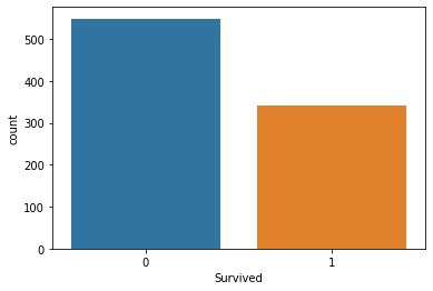
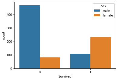
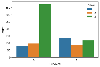
2.Visualization of various relationships between variables

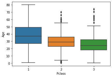
3. Using Box Plot to Get details about the distribution

sns.heatmap(titanic_data.isnull(), cbar=False)
sns.countplot(x=‘Survived’, data=titanic_data)
sns.countplot(x=‘Survived’, hue=‘Sex’, data=titanic_data)
sns.countplot(x=‘Survived’, hue=‘Pclass’, data=titanic_data)

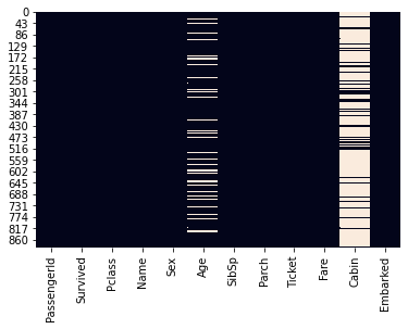
heatmap

Age and Cabin Have Null Entries

sns.boxplot(titanic_data[‘Pclass’], titanic_data[‘Age’])

Using function to replace null entries

def input_missing_age(columns):
age = columns[0]
passenger_class = columns[1]
if pd.isnull(age):
if(passenger_class == 1):
return titanic_data[titanic_data[‘Pclass’] == 1][‘Age’].mean()
elif(passenger_class == 2):
return titanic_data[titanic_data[‘Pclass’] == 2][‘Age’].mean()
elif(passenger_class == 3):
return titanic_data[titanic_data[‘Pclass’] == 3][‘Age’].mean()
else:
return age

Filling the missing Age data

titanic_data[‘Age’] = titanic_data[[‘Age’, ‘Pclass’]].apply(input_missing_age, axis = 1)

Drop null data

titanic_data.drop(‘Cabin’, axis=1, inplace = True)
titanic_data.dropna(inplace = True)

Create dummy variables for Sex and Embarked columns

sex_data = pd.get_dummies(titanic_data[‘Sex’], drop_first = True)
embarked_data = pd.get_dummies(titanic_data[‘Embarked’], drop_first = True)

Add dummy variables to the DataFrame and drop non-numeric data

titanic_data = pd.concat([titanic_data, sex_data, embarked_data], axis = 1)
titanic_data.drop([‘Name’, ‘PassengerId’, ‘Ticket’, ‘Sex’, ‘Embarked’], axis = 1, inplace = True)

Print the finalized data set

titanic_data.head()

Split the data set into x and y data

y_data = titanic_data[‘Survived’]
x_data = titanic_data.drop(‘Survived’, axis = 1)

Split the data set into training data and test data

from sklearn.model_selection import train_test_split
x_training_data, x_test_data, y_training_data, y_test_data = train_test_split(x_data, y_data, test_size = 0.3)

Create the model

from sklearn.linear_model import LogisticRegression
model = LogisticRegression()

Train the model and create predictions

model.fit(x_training_data, y_training_data)
predictions = model.predict(x_test_data)

Calculate performance metrics

from sklearn.metrics import classification_report
print(classification_report(y_test_data, predictions))

 precision    recall  f1-score   support

           0       0.83      0.87      0.85       169

           1       0.75      0.68      0.72        98

    accuracy                           0.80       267

   macro avg       0.79      0.78      0.78       267

weighted avg       0.80      0.80      0.80       267

Generate a confusion matrix

from sklearn.metrics import confusion_matrix
print(confusion_matrix(y_test_data,
predictions)

[[145  22]

 [ 30  70]]

With this, I finish this blog.
Hello Everyone, Namaste
My name is Pranshu Sharma and I am a Data Science Enthusiast
Thank you so much for taking your precious time to read this blog. Feel free to point out any mistake(I’m a learner after all) and provide respective feedback or leave a comment.
Dhanyvaad!!
Feedback:
Email: [email protected]

The media shown in this article are not owned by Analytics Vidhya and is used at the Author’s discretion.