This article was published as part of the Data Science Blogathon.
This guide entails concepts like ensemble learning, Voting Classifiers, a brief about bagging, pasting, and Out-of-bag Evaluation and their implementation. A brief about Random Forest, Extra Trees, and Feature Importance. Lastly, we will wrap things up by taking a quick look at Boosting and some basic QnAs.
Introduction to Ensemble Learning
Let’s start with an example, you have a question, and you ask it around, then aggregate their answers. In most cases, you would find that this answer is way better than one expert’s answer. So this is called the wisdom of the crowd. Similarly, if you aggregate the predictions of models such as classifiers or regressors, you would notice that the group has better performance than the best individual model. So this group of predictors or models are called ensemble and hence this technique is knowns as Ensemble learning.
For example, you can train a group of decision trees classifiers, on different random subsets of the training data. After that to make predictions, obtain predictions from all individual trees and predict the most frequent class (i.e predicted the most). This ensemble of decision trees is called Random Forest and is one of the most powerful algorithms in the machine learning world.
You will often use this technique, at the end of a project. Once you have a couple of good predictors in your hand and combine them even into a better one. Most of the winning solutions in machine learning competitions involve ensemble methods. (For example- Netflix’s prize competition).
So, go grab a coffee, make yourself comfortable. And let’s begin our journey of learning about Ensemble Learning.
Voting Classifiers in Ensemble Learning
Suppose you have a couple of classifiers, with each one having an accuracy of about 80-85%. Now, you can have a Support Vector Classifier, a Random Forest Classifier, a Logistics Regression Classifier, a K-Nearest Neighbors classifier, and perhaps a couple more. A simple way of creating an even better classifier is to combine the predictions of all classifiers and output the most frequent class. This type of classification(Majority-vote Classification) is known as Hard Voting Classifier.
The interesting part here is, this type of voting classifier often outperforms even the best classifier in the ensemble. In fact, even if each of the classifiers is a weak learner means it is slightly better than a model which is guessing randomly. The ensembles model can still be a strong learner, assuming there are enough weak learners and are independent of one another. An ensemble performs well only in cases when all the classifiers are perfectly independent of each other, i.e. making uncorrelated errors, which is quite challenging to achieve because they are all trained on the same data. Hence, they are likely to make the same types of errors. So in turn, there will be a majority of the votes for the wrong class, reducing the overall accuracy of the ensemble. One way to achieve a diverse set of classifiers is to use very different algorithms. With different algorithms, they may make different kinds of errors, which will in turn increase the accuracy of the ensemble.
The following code initializes and trains a classifier comprising three different classifiers which will be SVM, Random Forest, and Logistics Regression. We will be using Moon’s Dataset for our implementation.
Let’s start with our implementation
Importing necessary libraries:
from sklearn.model_selection import train_test_split
from sklearn.datasets import make_moons
from sklearn.linear_model import LogisticRegression
from sklearn.svm import SVC
from sklearn.ensemble import RandomForestClassifier
from sklearn.ensemble import VotingClassifier
from sklearn.metrics import accuracy_score
Creating dataset:
X, y = make_moons(n_samples=500, noise=0.30)
X_train, X_test, y_train, y_test = train_test_split(X, y)
Initializing the models:
log = LogisticRegression()
rnd = RandomForestClassifier(n_estimators=100)
svm = SVC()
voting = VotingClassifier(
    estimators=[('logistics_regression', log), ('random_forest', rnd), ('support_vector_machine', svm)],
    voting='hard')
Here we are setting voting = ‘hard’ means it will be following majority rule voting and n_estimators as 100. The rest of all the parameters are by default.
Fitting training data:
voting.fit(X_train, y_train)

Now let’s see how this works on the test set:
for clf in (log, rnd, svm, voting):
    clf.fit(X_train, y_train)
    y_pred = clf.predict(X_test)
    print(clf.__class__.__name__, accuracy_score(y_test, y_pred))

Boom! There we have it, as we can see the voting classifier outperforming other individual models slightly. If you are working with classifiers that have the predict_proba() method means they can estimate the probability of a class. Then, we output the class with the highest probability which is averaged over all the classifiers. This technique is knowns as soft voting. This technique usually performs better than hard voting as it focuses more on the highly confident votes. To use this, all you need to do is replace “hard” with “soft” and keep in mind that this will only work for the classifiers that can estimate the class probability.
Bagging and Pasting in Ensemble Learning
As discussed earlier, getting a diverse set of classifiers we can use different algorithms. There is another approach too, we can use the same algorithm for each predictor and train them on different random subsets of training data.
Bagging: Whenever we select a subset of the data with the replacement it is known as Bagging.
Pasting: Whenever we select a subset of the data without replacement it is known as Pasting.
Both bagging and pasting trains predictors on a different random subset of the training data. At the end, when all the predictors are trained, the ensemble can predict new data by simply combining the prediction of all the predictors the same as the hard voting classifier(As mode in statistics). Most of the time ensemble has the same bias but less variance than an individual predictor trained on the original training data.
For more information on Bias and Variance check out this blog here.
The biggest advantage of bagging and pasting is that can they can be trained to different CPUs or on different servers as well and this is one of many other reasons why both are very popular methods.
Let’s start with our implementation:
We will be using the same dataset that we created earlier.
Importing necessary libraries:
from sklearn.ensemble import BaggingClassifier
from sklearn.tree import DecisionTreeClassifier
from sklearn.metrics import accuracy_score
Initializing a bagging classifier:
bagging_clf = BaggingClassifier(
    DecisionTreeClassifier(), n_estimators=250,
    max_samples=100, bootstrap=True, random_state=101)
Let’s break down the code a little bit here, the above code will train an ensemble of 250 decision tree classifiers(n_estimators), and each of them is trained on 100 random subsets of the training data(max_samples)with replacement as we are working on a bagging classifier but if you wish to work on pasting instead, go ahead and set the bootstrap = False. Lastly, the n_jobs parameters specify how many CPU cores you want to use for training and prediction(-1 means it can use all available). For regression, you can use BaggingRegressors.
Check out the official documentation here for more information.
Training the classifier:
bagging_clf.fit(X_train, y_train)
Testing the classifier:
y_pred = bagging_clf.predict(X_test)
print(accuracy_score(y_test, y_pred))

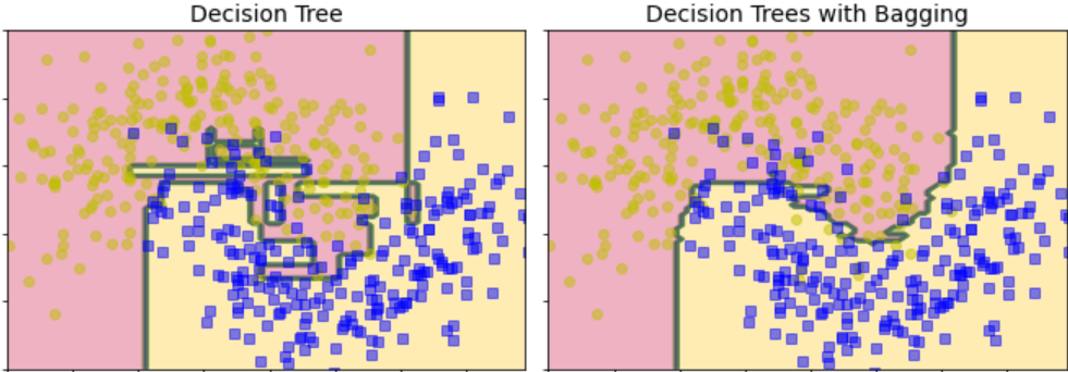
If we compare a regular decision tree classifier with the bagging classifier we just created, both of them are trained on moons dataset. By observing, the below figure we can see that

The ensemble is much more generalized than an individual decision tree.
Out-Of-Bag Evaluation
Whenever you use bagging, there is some amount of data that might be sampled(selecting subset) more than once, or perhaps even more and there might be some data that is not sampled at all. Bagging Classifier samples n training instances with replacement by default, which means only around 63% of data is sampled on an average for each predictor. The rest of the 37% of the data are not sampled at all, now these data/instances are knowns as out-of-bag(OOB) instances. Remember this 37% are not the same for all predictors.
Since our model never saw this data before, it can be useful for evaluating removing the need for separate validation data.
Bagging classifier has a parameter oob_score which upon setting true will automatically use oobs for evaluation after training is done.
Let’s get a quick look at the implementation:
The libraries and datasets used here are the same.
Initializing the classifier:
bagging_clf = BaggingClassifier(
    DecisionTreeClassifier(), n_estimators=250,
    bootstrap=True, oob_score=True, random_state=101)
Training the Classifier:
bagging_clf.fit(X_train, y_train)
Result:
bagging_clf.oob_score_

Rounding it off we get 90% which is close enough to what we achieved earlier(91.2%). So by testing the model on oobs we can get a rough estimate of the accuracy we will achieve on the test set.
Random Forests
As we have already discussed in the introduction, the Random forest is just an ensemble of decision trees trained by the bagging method. Here, the max_Samples are set to the size of training data. So instead of creating a bagging classifier using decision trees, it is better for you to straight away use the RandomForest Classifier or RandomForest Regressor(for regression) which is way more optimized and efficient to use.
Let’s take a quick look at the implementation:
Importing necessary libraries:
from sklearn.ensemble import RandomForestClassifier
Initialize and training(same moon’s dataset):
random_forest_clf = RandomForestClassifier(n_estimators=500, max_leaf_nodes=16, random_state=42,n_jobs=-1)
random_forest_clf.fit(X_train, y_train)
The above code trains a Random Forest Classifier with 500 trees(n_estimators=500) and uses all available CPU cores, as we have specified n_jobs =-1, each of them limited to a maximum of 16 nodes.
For more in detail information on Decision Tree, Check it out here.
Predicting for test data:
y_pred_random_forest = random_forest_clf.predict(X_test)
Random Forest Classifier consists of all the hyperparameters of a Decision Tree Classifier as well as that of Bagging Classifier to control the process.
The Random Forest algorithm uses extra randomness when growing trees. Instead of searching for the best feature while splitting the node. What it does is, searches for the best feature among a random subset of features. The algorithm also trades a higher bias for a lower variance, in turn increasing the overall accuracy.
Let’s go ahead and create a similar Bagging classifier and compare its predictions with that of the Random Forest Classifier.
Initializing and training the model:
bagging_clf = BaggingClassifier(
    DecisionTreeClassifier(max_leaf_nodes=16),
    n_estimators=500, random_state=101)
Training and Predicting:
bagging_clf.fit(X_train, y_train)
y_pred_bagging = bagging_clf.predict(X_test)
Now, let’s compare predictions of the bagging classifier(y_pred_bagging) and Random Forest(y_pred_random_forest) see what we get:
np.sum(y_pred_bagging == y_pred_random_forest) / len(y_pred_bagging)

As we can see almost 95.2% of predictions of the Bagging classifier and Random Forest are similar.
Extra Trees
Let’s go ahead with this topic briefly.
Whenever the Random Forest grows a tree, for each node only a random subset of features is taken into the account for splitting. One way of making tress even more random is by setting the random threshold for each feature instead of searching for the best threshold like the decision tree does.
This technique also trades high bias for low variance. The advantage of using Extra trees instead of a random forest is that it is faster, as finding the best possible threshold for each feature at every node is extremely time-consuming.
The creation of the Extra trees classifier is almost similar to that of the Random Forest Classifier. For Classification, you can use Scikit-learn’s Extra Trees classifier class, and for regression Scikit-learn’s Extra Tree Regressor class.
It is difficult to know which would perform better or worst among random forests and extra trees, the only way for you to know is to create both and compare them using cross-validation.
Feature Importance
By far one of the best things that Random Forest has to offer, it helps us to measure the importance of each every feature. Scikit-learn calculates it by analyzing how much a tree node that uses that feature reduces impurity on average.
Scikit-learn automatically calculates these scores for each and every feature and after that scales it so that the sum of all importance is equal to 1. To access the importance of the feature we will be using the feature_importances variable.
Let take a look at the implementation part for both IRIS and MNIST datasets:
IRIS DATASET
Import necessary libraries and load dataset:
from sklearn.datasets import load_iris
iris = load_iris()
Initialize and train a Random Forest Classifier:
rand_forest_clf = RandomForestClassifier(n_estimators=500, random_state=42)
rand_forest_clf.fit(iris["data"], iris["target"])
Print the feature importance along with their names respectively:
for feature, score in zip(iris["feature_names"], rand_forest_clf.feature_importances_):
    print(feature, score)


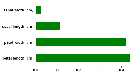
Here we can observe that petal length(44%) and petal width(42%) seem to have greater importance than sepal length(11%) and sepal width(2%).
MNIST DATASET
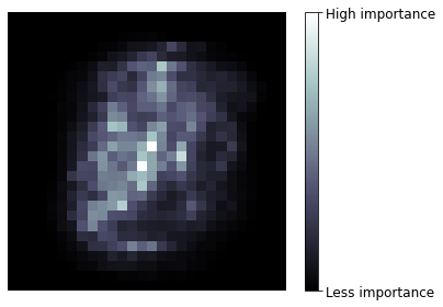
Let’s go ahead and train random Forest Classifier on the MNIST dataset and plot each pixel’s importance using matplotlib.
Initializing and training the model:
rand_forest_clf = RandomForestClassifier(n_estimators=100, random_state=42)
rand_forest_clf.fit(mnist["data"], mnist["target"])
Instead of printing the feature importance, it is better to straightway visualize it:
image = rand_forest_clf.feature_importances_.reshape(28, 28)
plt.imshow(image, cmap = mpl.cm.bone,interpolation="nearest")
plt.axis("off")
cbar = plt.colorbar(ticks=[rand_forest_clf.feature_importances_.min(), rand_forest_clf.feature_importances_.max()])
cbar.ax.set_yticklabels(['Less importance', 'High importance'])
plt.show()

It is pretty simple to interpret that the boundaries of the images have no significance in the prediction of a particular number.
If you have fond of Visualization, do check out my blog here.
So if you need to perform feature selection, Random forest is there to help you to get a quick analysis of which features matter a lot.
Boosting
Whenever several weak learners are combined to form a strong learner, we call it boosting(boosting hypothesis). Basically what it does is train the predictors in sequential order, each of them corrects its predecessor’s mistake. There are lots of boosting algorithms Scikit-learn has to offer but by far the best and the most popular ones are AdaBoost(Adaptive Boosting) and Gradient Boosting.
Let’s break down Adaboost first:
AdaBoost
Generally, the technique used by AdaBoost is it pays attention to the training data its predecessors under fitted. This results in new predictors concentrating more on these hard cases.
Let’s understand this with an example. When training an Adaboost classifier, the algorithm first trains a base classifier(suppose Decision Trees) and after training it uses this base classifier to make predictions on the training data. After this, the algorithm then increases its relative weight for the training instances which our base classifier got wrong(misclassification). Then it trains another classifier with these new(updated) weights and again makes predictions on training data, and updates its weights accordingly, and this process goes on and on.
Once all the predictors are trained and good to go, the ensemble makes predictions similar to bagging or pasting, the only difference is that the predictors have different weights according to the accuracy(classifications that they got right) on the training data.
One of the major drawbacks of this sequential approach is that they cannot be parallelized meaning they cannot be trained on different systems at the same time as each of the predictors requires the training and evaluation of its previous predictors. Hence, they don’t scale like bagging and pasting.
We won’t be discussing the mathematics behind this but I request you to check out some other blogs or articles to get a mathematical intuition and an in detail overall working.
Let’s get a quick look at the implementation:
The dataset is the same that we created before, in case you forgot; since you are a long way down 🙂
from sklearn.ensemble import AdaBoostClassifier
adaboost_clf = AdaBoostClassifier(
    DecisionTreeClassifier(max_depth=1), n_estimators=200,
    algorithm="SAMME.R", learning_rate=0.5, random_state=42)
adaboost_clf.fit(X_train, y_train)
The above code trains an AdaBoost classifier based on 200 Decision Stumps(one withmax_depth set to 1, consists of a single decision node and two leaf nodes). Here learning rate is the weight applied to each classifier during the boosting iterations. The higher the learning rate, the higher is the contribution of each classifier. Keep in mind that there is a trade between n_estimators and learning rate.
Now you must be wondering what is SAMME here, so it is a multi-class version of AdaBoost which stands for Stagewise Addictive Modelling using a Multiclass Exponential Loss function. You might have also noticed an (.R) there, it stands for real, if the predictors with which you are working have the predict_proba() method meaning they can estimate class probabilities, you can use a. R because class probabilities generally perform better. This is the default base estimator for AdaBoost Classifier.
Prediction and Accuracy:
y_pred = adaboost_clf.predict(X_test)
accuracy_score(y_test, y_pred)

We got around 90% of accuracy, which is too not bad!
Now let’s start with Gradient Boosting.
Gradient Boosting
The second extremely popular boosting algorithm we are about to see is gradient boosting. Gradient boost also works pretty much the same way as AdaBoost works i.e. sequentially adding predictors to an ensemble, with each one of them correcting its predecessor. The only difference is that instead of tweaking the weights at every iteration like AdaBoost, this method focuses more on and tries to fit new predictors to the residual error made by the previous one.
Residual error in simple terms means the difference between a group of values observed and their arithmetic mean.
Let’s go with a simple example for better understanding:
We will be using a decision tree as a base predictor. Let’s go ahead and fit a decision tree regressor to the training data. We will change the dataset now, here we will create a simple noisy quadratic dataset.
np.random.seed(42)
X = np.random.rand(100, 1) - 0.5
y = 3*X[:, 0]**2 + 0.05 * np.random.randn(100)
As our dataset creation is complete let’s go ahead and fit it into our model.
from sklearn.tree import DecisionTreeRegressor
tree_reg_first = DecisionTreeRegressor(max_depth=2, random_state=42)
tree_reg_first.fit(X, y)
As discussed earlier, that this method focuses on residual errors. Now we will train the second decision tree regressor on the residual errors by the first one.
y2 = y - tree_reg_first.predict(X)
tree_reg_second = DecisionTreeRegressor(max_depth=2, random_state=42)
tree_reg_second.fit(X, y2)
We need to train the third regressor using the residuals made by the previous (second) one.
y3 = y2 - tree_reg_second.predict(X)
tree_reg_third = DecisionTreeRegressor(max_depth=2, random_state=42)
tree_reg_third.fit(X, y3)
Now let’s create an ensemble consisting of all the trees we just trained.
X_new = np.array([[0.8]]) //value on which we will test it.
y_pred = sum(tree.predict(X_new) for tree in (tree_reg_first, tree_reg_second, tree_reg_third))
Now it will make predictions for new data by just adding up a prediction of all the trees. Let’s go ahead and see what it predicts.
y_pred

So it predicted y = 0.75 for x = 0.8.
The following code works pretty much the same way:
from sklearn.ensemble import GradientBoostingRegressor
gbrt = GradientBoostingRegressor(max_depth=2, n_estimators=3, learning_rate=1.0, random_state=42)
gbrt.fit(X, y)
And it will create the same ensembles as the ones which looked earlier.
gbrt.predict(X_new)

Check out the official documentation for more info.
Ensemble Learning Q&A Session
In this section, we will go through some basic questions so you can get a tighter hold on the topics we just discussed.
1. What is the difference between hard and soft voting classifiers?
Answer: A hard voting classifier just counts the votes of each classifier in the ensemble and outputs the class which was in majority. On the other hand, a soft voting classifier calculates the class probability for each classifier in the ensemble and outputs the class with the highest probability. But soft voting only works for the classifier which has the predict_proba() method.
2. Do you think you can speed up the training time of bagging by distributing it across multiple servers? If yes, then why? What about Pasting, boosting, and Random Forest?
Answer: Yes it is possible to speed up the training time of bagging by distributing them on multiple servers because all of them are independent of each other. Pasting and Random Forest also works similarly. So no issue with them too. Talking about boosting algorithms they rely on their predecessors. So it is not possible to train them across multiple servers.
3. What are the advantages of Out-Of-Bag Evaluation?
Answer: As we all know that in the out-of-bag evaluation, each predictor is evaluated on the instances on which it was not trained (37% that were left, if you remember). This gives an advantage of having an unbiased evaluation of the ensemble without any need for a validation set.
4. How are Extra Trees any different from a Regular Random Forest? Between Extra Trees and random Forest which is faster? How can Randomness help in extra trees?
Answer: Both Extra Trees and Random Forest considers a random subset of features for splitting at each node. The only difference is that instead of searching for the best possible threshold for a feature, extra trees use a random threshold. This randomness of features acts as regularization, if ever Random Forest is overfitting the training data there is a good chance that Extra trees might perform better. In terms of prediction speed, both of them are the same, as we know that Extra Trees don’t look for the best threshold for a feature, it saves it a lot of time. Hence, making it faster than Random Forest.
5. While working you find that the AdaBoost classifier is underfitting the training data, what are the hyperparameters you will tweak, and how?
Answer: If we observe that AdaBoost is underfitting the training data, we can try on increasing the number of estimators or we can also try reducing the regularization hyperparameters of the base estimator. Increasing the learning rate might also help a bit.
6. While working you find that your Gradient Boosting is overfitting the training data, what are your thoughts about the learning rate?
Answer: If we observe that Gradient Boosting is overfitting the training data, we can go ahead and reduce the learning rate, and also we can use early stopping (another hot topic will discuss some other day) to find the right number of predictors.
So if you got half of or all of the above questions right, congratulation! You probably have gone through all of the paragraphs of this guide. I’m Grateful to have a reader like you…
Endnotes
Finally, our journey of learning this topic has come to an end!. It was quite a long one. But glad to have you with me throughout. To wrap things up… let’s revise the topics that we saw in this guide. Firstly, we started with a general introduction, then some basic discussion about voting classifiers, we saw what is bagging, pasting, and out-of-bag evaluation along with their implementation, then we saw a brief working of Random Forest, Extra-Trees and Features importance theoretically as well as practically, lastly, we gave a glance on boosting algorithms. We also got a chance to go through some questions, through which you can assess yourself about how much you were able to consume in this guide.
Stay tuned!!
Check out my other blogs here.
I hope you enjoyed reading this article, if you found it useful, please share it among your friends on social media too. For any queries and suggestions feel free to ping me here in the comments or you can directly reach me through email.
Connect me with on LinkedIn
Email: [email protected]
Thank You!
The media shown in this article is not owned by Analytics Vidhya and are used at the Author’s discretion.


