This article was published as a part of the Data Science Blogathon.
A Tour of Evaluation Metrics for Machine Learning
After we train our machine learning, it’s important to understand how well our model has performed. Evaluation metrics are used for this same purpose. Let us have a look at some of the metrics used for Classification and Regression tasks.
Classification Evaluation Metrics
Classification evaluation metrics score generally indicates how correct we are about our prediction. The higher the score, the better our model is.
Before diving into the evaluation metrics for classification, it is important to understand the confusion matrix.
Confusion Matrix:
A confusion matrix is a technique for summarizing the performance of a classification algorithm.
A few terms associated with the confusion matrix are
-
True positive: An instance for which both predicted and actual values are positive.
-
True negative: An instance for which both predicted and actual values are negative.
-
False Positive: An instance for which predicted value is positive but actual value is negative.
-
False Negative: An instance for which predicted value is negative but actual value is positive.
A confusion matrix follows the below format:

Example: Cancer Detection:
Consider a problem where we are required to classify whether a patient has cancer or not.
In the below table the columns represent the rows that present the number of predicted values and the columns present the number of actual values for each class. There are 500 total instances. This is the example we will use throughout the blog for classification purposes. Below is the confusion matrix.

Note Post this point in the blog, I’ll refer to True positive as TP, False positive as FP, True Negative as TN, and False Negative as FN.
For the above confusion matrix
Number of TP:7
Number of TN: 480
Number of FP: 8
Number of FN: 5
Accuracy:
Accuracy can be defined as the percentage of correct predictions made by our classification model.
The formula is:
Accuracy = Number of Correct predictions/number of rows in data
Which can also be written as:
Accuracy = (TP+TN)/number of rows in data
So, for our example:
Accuracy = 7+480/500 = 487/500 = 0.974.
Our model has a 97.4% prediction accuracy, which seems exceptionally good.
Accuracy is a good metric to use when the classes are balanced, i.e proportion of instances of all classes are somewhat similar. However, it is to be noted that accuracy is not a reliable metric for datasets having class imbalance, i.e The total number of instances of a class of data is far less than the total number of instances for another class of data. In this case, the number of positives in the dataset is 12 (TP+FN = 7+ 5 = 12) and the number of negatives is 488. Since we are dealing with an imbalanced class problem, it’s better to check our performance on other metrics before concluding our model’s performance.
Precision:
Precision indicates out of all positive predictions, how many are actually positive. It is defined as a ratio of correct positive predictions to overall positive predictions.
Precision = Predictions actually positive/Total predicted positive.
Precision = TP/TP+FP
For our cancer detection example, precision will be 7/7+8 = 7/15 = 0.46
Recall:
Recall indicates out of all actually positive values, how many are predicted positive. It is a ratio of correct positive predictions to the overall number of positive instances in the dataset.
Recall = Predictions actually positive/Actual positive values in the dataset.
Recall = TP/TP+FN
For our cancer detection example, recall will be 7/7+5 = 7/12 = 0.58
As we can see, the precision and recall are both lower than accuracy, for our example.
Deciding whether to use precision or recall:
It is mathematically impossible to increase both precision and recall at the same time, as both are inversely proportional to each other.. Depending on the problem at hand we decide which of them is more important to us.
We will first need to decide whether it’s important to avoid false positives or false negatives for our problem. Precision is used as a metric when our objective is to minimize false positives and recall is used when the objective is to minimize false negatives. We optimize our model performance on the selected metric.
Below are a couple of cases for using precision/recall.
-
An AI is leading an operation for finding criminals hiding in a housing society. The goal should be to arrest only criminals, since arresting innocent citizens can mean that an innocent can face injustice. However, if the criminal manages to escape, there can be multiple chances to arrest him afterward. In this case, false positive(arresting an innocent person) is more damaging than false negative(letting a criminal walk free). Hence, we should select precision in order to minimize false positives.
-
We are all aware of the intense security checks at airports. It is of utmost importance to ensure that people do not carry weapons along them to ensure the safety of all passengers. Sometimes these systems can lead to innocent passengers getting flagged, but it is still a better scenario than letting someone dangerous onto the flight. Each flagged individual is then checked thoroughly once more and innocent people are released. In this case, the emphasis is on ensuring false negatives(people with weapons getting into flights) are avoided during initial scanning, while detected false positives(innocent passengers flagged) are eventually let free. This is a scenario for minimizing false negatives and recall is the ideal measure of how the system has performed.
F1 score:
Consider a scenario where your model needs to predict if a particular employee has to be promoted or not and promotion is the positive outcome. In this case, promoting an incompetent employee(false positive) and not promoting a deserving candidate(false negative) can both be equally risky for the company.
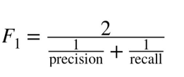
When avoiding both false positives and false negatives are equally important for our problem, we need a trade-off between precision and recall. This is when we use the f1 score as a metric. An f1 score is defined as the harmonic mean of precision and recall.
Formula:
Threshold:
Any machine learning algorithm for classification gives output in the probability format, i.e probability of an instance belonging to a particular class. In order to assign a class to an instance for binary classification, we compare the probability value to the threshold, i.e if the value is greater than or less than the threshold.
For probability >= threshold, class = 1
probability < threshold, class = 0
For multi-class classification, we can assign the class for which the instance has maximum probability value as the final class value.
AUC-ROC:
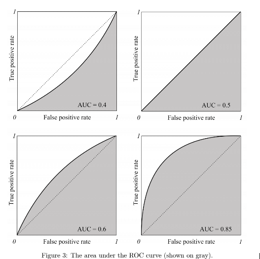
We use the receiver operating curve to check model performance. Wikipedia defines ROC as: “A receiver operating characteristic curve, or ROC curve, is a graphical plot that illustrates the diagnostic ability of a binary classifier system as its discrimination threshold is varied”. Below is an example:
Reference: [1]
The x-axis represents the false positive rate and the y-axis represents the true positive rate.
True Positive Rate is also known as recall and False positive rate is the proportion of negative examples predicted incorrectly, both of them have a range of 0 to 1. Below are the formulas:
True Positive Rate(tpr) = TP/TP+FN
False Positive Rate(fpr) = FP/FP+TN
The shaded region is the area under the curve(AUC). Mathematically the roc curve is the region between the origin and the coordinates(tpr,fpr).
The higher the area under the curve, the better the performance of our model. We can improve the AUC-ROC score by changing true and false-positive rates, which in turn can be changed using the threshold value.
Regression Evaluation Metrics
Unlike classification, where we measure a model’s performance by checking how correct it’s predictions are, in regression we check it by measuring the difference in predicted and actual values, our objective is to minimize the metric score in order to improve our model. We will use the below example to understand more.
Example:
Below is the example we will use, the difference between the actual and predicted value is the error our model makes during prediction.
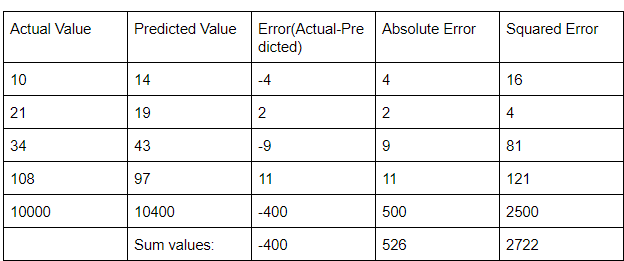
Number of samples(N) = 5.
When we add the error values (containing both positive and negative values) these elements cancel out each other and we may get an error value lower than it should be. For example, in the first 4 rows of our example -4+2-9+11 = 0. The sum of differences, i.e error will be 0. However, we can clearly see that none of the 4 rows got the prediction correct. This can lead to a problem when calculating the effectiveness of the model. In order to mitigate this issue, we use other evaluation metrics.
Mean Absolute Error:
As the name suggests the mean absolute error can be defined as the mean of the sum of absolute differences between the predicted and actual values of the continuous target variable.
MAE = Σ | y_actual – y_predicted | / n
For our example, MAE will be 526/5 = 105.2
Mean Squared Error:
There can be instances where large errors are undesirable. Let’s say that one of the predictions of a model is an outlier. In this case, we should penalize this higher error to a greater extent. Which is where we can use mean squared error.
The average of the sum of squares of differences between the predicted and actual values of the continuous target variable.
MSE = Σ (y_actual – y_predicted)2 / n
For our example, mse will be 544.4
Root Mean Squared Error:
The metric of the attribute changes when we calculate the error using mean squared error. For e.g, if the unit of a distance-based attribute is meters(m) the unit of mean squared error will be m2, which could make calculations confusing. In order to avoid this, we use the root of mean squared error.
RMSE = √MSE = √ Σ (y_actual – y_predicted)2 / n
For our example, rmse will be 23.33
R-Squared
In classification, where metrics output a value between 0 to 1, and the score can be used to objectively judge a model’s performance. However, in regression the target variable may not always be in the same range, e.g the price of a house can be a 6 digits number but a student’s exam marks in a subject are between 0-100. This means that the metric scores for marks will mostly be a 2 digit number, but that for housing prices can be anything between a 1-6 digit number.
In simpler words, an accuracy of 0.90 or 90% is a good performance, but does an RMSE of 90 indicate good performance. For house price which is a 6 digit number, it’s a good score, but for a student’s marks, it is a terrible one! Predicting a value of 10, when the actual value is 100 is much different than predicting a value of 200,000 when the actual value is 200,090.
R-squared acts as a benchmark metric for judging a regression model’s performance, irrespective of the range of values the target variable presents. The range of r-squared is between 0 and 1. The greater the r-squared value the better our model’s performance is.
When new features are added to data, the R-squared value either increases or remains the same. However, adding features does not always guarantee a better performance for the model and r-squared fails to adequately capture the negative impact of adding a feature to our model, i.e whether the feature actually improves model predictions or not. In order to address this problem, the adjusted r-squared metric is used.
Before we get into the formula, let’s look into what Residual sum of squares and the total sum of squares.
Residual sum of squares(RSS):
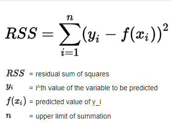
RSS is defined as the sum of squares of the difference between the actual and predicted values. Below is the formula
Reference:[2]
Total sum of squares(TSS):
TSS is defined as the sum of squares of the difference between the mean value and actual values. Below is the formula
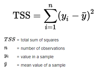
Reference:[2]
The formula for r-squared will be:
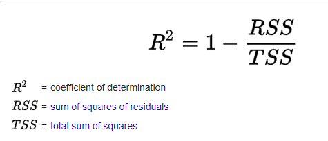
Reference:[2]
Adjusted R-Squared:
The only difference between r-squared and adjusted r-squared is that the adjusted r-squared value increases only if the feature added improves the model performance, thus capturing the impact of adding features more adequately. Below is the formula for adjusted r-squared

Reference: [3]
Conclusion:
The selection of the right evaluation metrics is a very important part of machine learning. Hope this article has helped to improve your understanding of it.


