Introduction
Machine learning is connected with the field of education related to algorithms which continuously keeps on learning from various examples and then applying them to real-world problems. Classification is a task of Machine Learning which assigns a label value to a specific class and then can identify a particular type to be of one kind or another. The most basic example can be of the mail spam filtration system where one can classify a mail as either “spam” or “not spam”. You will encounter multiple types of classification challenges and there exist some specific approaches for the type of model that might be used for each challenge.
Classification Predictive Modeling in Machine Learning
Classification usually refers to any kind of problem where a specific type of class label is the result to be predicted from the given input field of data. Some types of Classification challenges are :
- Classifying emails as spam or not
- Classify a given handwritten character to be either a known character or not
- Classify recent user behaviour as churn or not
For any model, you will require a training dataset with many examples of inputs and outputs from which the model will train itself. The training data must include all the possible scenarios of the problem and must have sufficient data for each label for the model to be trained correctly. Class labels are often returned as string values and hence needs to be encoded into an integer like either representing 0 for “spam” and 1 for “no-spam”.

Image 1
There is no general theory for the best model but one is expected to experiment and discover which algorithm and configuration will result in the best performance for a specific task. In classification predictive modelling, the various algorithms are compared with their results. Classification accuracy is an interesting metric to evaluate the performance of any model based on the various predicted class labels. Classification accuracy might not be the best parameter but is a good point to begin for most of the classification tasks.
In place of a class label, some might give us the prediction of a probability of class membership of a particular input and in such cases, the ROC curve can be a helpful indicator of how accurate one model is. There are mainly 4 different types of classification tasks that you might encounter in your day to day challenges. Generally, the different types of predictive models in machine learning are as follows :
- Binary classification
- Multi-Label Classification
- Multi-Class Classification
- Imbalanced Classification
We will go over them one by one.
Binary Classification for Machine Learning
A binary classification refers to those tasks which can give either of any two class labels as the output. Generally, one is considered as the normal state and the other is considered to be the abnormal state. The following examples will help you to understand them better.
- Email Spam detection: Normal State – Not Spam, Abnormal State – Spam
- Conversion prediction: Normal State – Not churned, Abnormal State – Churn
- Conversion Prediction: Normal State – Bought an item, Abnormal State – Not bought an item
You can also add the example of that ” No cancer detected” to be a normal state and ” Cancer detected” to be the abnormal state. The notation mostly followed is that the normal state gets assigned the value of 0 and the class with the abnormal state gets assigned the value of 1. For each example, one can also create a model which predicts the Bernoulli probability for the output. You can read more about the probability here. In short, it returns a discrete value that covers all cases and will give the output as either the outcome will have a value of 1 or 0. Hence after the association to two different states, the model can give an output for either of the values present.
The most popular algorithms which are used for binary classification are :
- K-Nearest Neighbours
- Logistic Regression
- Support Vector Machine
- Decision Trees
- Naive Bayes
Out of the mentioned algorithms, some algorithms were specifically designed for the purpose of binary classification and natively do not support more than two types of class. Some examples of such algorithms are Support Vector Machines and Logistic Regression. Now we will create a dataset of our own and use binary classification on it. We will use the make_blob() function of the scikit-learn module to generate a binary classification dataset. The example below uses a dataset with 1000 examples that belong to either of the two classes present with two input features.
Code :
The above example creates a dataset of 5000 samples and divides them into input ‘X’ and output ‘Y’ elements. The distribution shows us that anyone instance can either belong to either class 0 or class 1 and there are approximately 50% in each.
The first 10 examples in the dataset are shown with the input values which are numeric and the target value is an integer which represents a class membership.
Then a scatter plot is created for the input variables where the resultant points are colour coded based on the class value. We can easily see two distinct clusters which we can discriminate.
Multi-Class Classification
These types of classification problems have no fixed two labels but can have any number of labels. Some popular examples of multi-class classification are :
- Plant Species Classification
- Face Classification
- Optical Character recognition
Here there is no notion of a normal and abnormal outcome but the result will belong to one of many among a range of variables of known classes. There can also be a huge number of labels like predicting a picture as to how closely it might belong to one out of the tens of thousands of the faces of the recognition system.
Another type of challenge where you need to predict the next word of a sequence like a translation model for text could also be considered as multi-class classification. In this particular scenario, all the words of the vocabulary define all the possible number of classes and that can range in millions.
These types of models are generally done using a Categorical Distribution unlike Bernoulli for binary classification. In a Categorical Distribution, an event can have multiple endpoints or results and hence the model predicts the probability of input with respect to each of the output labels.
The most common algorithms which are used for Multi-Class Classification are :
- K-Nearest Neighbours
- Naive Bayes
- Decision trees
- Gradient Boosting
- Random Forest
You can also use the algorithms for Binary Classification here on a basis of either one class vs all the other classes, also known as one-vs-rest, or one model for a pair of classes in the model which is also known as one-vs-one.
One Vs Rest – The main task here is to fit one model for each class which will be versus all the other classes
One Vs One – The main task here is to define a binary model for every pair of classes.
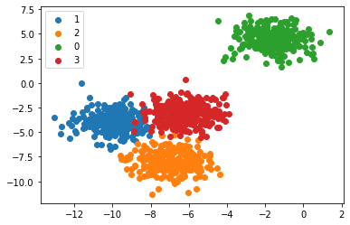
We will again take the example of multi-class classification by using the make_blobs() function of the scikit learn module. The following code demonstrates it.
Code :
from numpy import where
from collections import Counter
from sklearn.datasets import make_blobs
from matplotlib import pyplot
X, y = make_blobs(n_samples=1000, centers=4, random_state=1)
print(X.shape, y.shape)
counter = Counter(y)
print(counter)
for i in range(10):
  print(X[i], y[i])
for label, _ in counter.items():
  row_ix = where(y == label)[0]
  pyplot.scatter(X[row_ix, 0], X[row_ix, 1], label=str(label))
pyplot.legend()
pyplot.show()
Output :
(1000, 2) (1000,)
Counter({1: 250, 2: 250, 0: 250, 3: 250})
[-10.45765533  -3.30899488] 1
[-5.90962043 -7.80717036] 2
[-1.00497975  4.35530142] 0
[-6.63784922 -4.52085249] 3
[-6.3466658  -8.89940182] 2
[-4.67047183 -3.35527602] 3
[-5.62742066 -1.70195987] 3
[-6.91064247 -2.83731201] 3
[-1.76490462  5.03668554] 0
[-8.70416288 -4.39234621] 1

Here we can see that there are more than two class types and we can classify them separately into the different types.
Multi-Label Classification for Machine Learning
In multi-label Classification, we refer to those specific classification tasks where we need to assign two or more specific class labels that could be predicted for each example. A basic example can be photo classification where a single photo can have multiple objects in it like a dog or an apple and etcetera. The main difference is the ability to predict multiple labels and not just one.
You cannot use a binary classification model or a multi-class classification model for multi-label classification and you have to use a modified version of the algorithm to incorporate for multiple classes which can be possible and then to look for them all. It becomes more challenging than a simple yes or no statement. The common algorithms used here are :
- Multi-label Random Forests
- Multi-label Decision trees
- Multi-label Gradient Boosting
One more approach is to use a separate classification algorithm for the label prediction for each and every type of class. We will use a library from scikit-learn to generate our multi-label classification dataset from scratch. The following code creates and shows the working example of multi-label classification of 1000 samples and 4 types of classes.
Code:
from sklearn.datasets import make_multilabel_classification
X, y = make_multilabel_classification(n_samples=1000, n_features=3, n_classes=4, n_labels=4, random_state=1)
print(X.shape, y.shape)
for i in range(10):
	print(X[i], y[i])
Output :
(1000, 3) (1000, 4)
[ 8. 11. 13.] [1 1 0 1]
[ 5. 15. 21.] [1 1 0 1]
[15. 30. 14.] [1 0 0 0]
[ 3. 15. 40.] [0 1 0 0]
[ 7. 22. 14.] [1 0 0 1]
[12. 28. 15.] [1 0 0 0]
[ 7. 30. 24.] [1 1 0 1]
[15. 30. 14.] [1 1 1 1]
[10. 23. 21.] [1 1 1 1]
[10. 19. 16.] [1 1 0 1]
Imbalanced Classification for Machine Learning
An Imbalanced Classification refers to those tasks where the number of examples in each of the classes are unequally distributed. Generally, imbalanced classification tasks are binary classification jobs where a major portion of the training dataset is of the normal class type and a minority of them belong to the abnormal class.
The most important examples of these use cases are :
- Fraud Detection
- Outlier Detection
- Medical Diagnosis Test
The problems are transformed into binary classification tasks with some specialized techniques. You can either utilise undersampling for the majority classes or oversampling for the minority classes. The most prominent examples are :
- Random Undersampling
- SMOTE Oversampling
Special modelling algorithms can be used to give more attention to the minority class when the model is being fitted on the training dataset which includes cost-sensitive machine learning models. Especially for cases like :
- Cost-Sensitive Logistic Regression
- Cost-Sensitive Decision Trees
- Cost-Sensitive Support Vector Machines
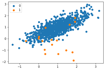
So after choosing the model, we need to access the model and score it for which we can either use Precision, Recall or F-Measure score. Now we will take a look to develop a dataset for the imbalanced classification problem. We will use the Classification function of scikit-learn to generate a fully synthetic and imbalanced binary classification dataset of 1000 samples
Code :
from numpy import where
from collections import Counter
from sklearn.datasets import make_classification
from matplotlib import pyplot

X, y = make_classification(n_samples=1000, n_features=2, n_informative=2, n_redundant=0, n_classes=2, n_clusters_per_class=1, weights=[0.99,0.01], random_state=1)
print(X.shape, y.shape)
counter = Counter(y)
print(counter)
for i in range(10):
print(X[i], y[i])
for label, _ in counter.items():
row_ix = where(y == label)[0]
pyplot.scatter(X[row_ix, 0], X[row_ix, 1], label=str(label))
pyplot.legend()
pyplot.show()
Output :
(1000, 2) (1000,)
Counter({0: 983, 1: 17})
[0.86924745 1.18613612] 0
[1.55110839 1.81032905] 0
[1.29361936 1.01094607] 0
[1.11988947 1.63251786] 0
[1.04235568 1.12152929] 0
[1.18114858 0.92397607] 0
[1.1365562  1.17652556] 0
[0.46291729 0.72924998] 0
[0.18315826 1.07141766] 0
[0.32411648 0.53515376] 0

Here we can see the distribution of the labels and we can see a severe imbalance of the classes where 983 elements belong to one type and only 17 belong to the other type. We can see a majority of type 0 or class 0 as expected. These types of datasets are more difficult to identify but they have a more general and practical use case.
Conclusion
Thank you for reading till the end of the article and if you find it helpful in any way, don’t forget to share it with your network. If you would want to read some of the other articles by me, you can click here and feel free to connect with me on LinkedIn or Github.
References
- Link to the Collab Document : https://colab.research.google.com/drive/1EiGZCGypDIHFNuzm71QN16NJxas41vE3?usp=sharing
- Arnab Mondal – Data Engineer | Python, C/C++, AWS Developer | Freelance Tech Writer
Image Sources
- Image 1 – https://unsplash.com/photos/n6B49lTx7NM
The media shown in this article are not owned by Analytics Vidhya and are used at the Author’s discretion.


