Hello there, guys! Good day, everyone! Today we’ll look at an intriguing issue in data pre-processing: how to deal with missing values (which is part of Data Cleaning). So, before we get into the meat of the matter, let’s review some fundamental terminology so that we can see why we need to be concerned about missing values. The subjects that we will explore in this thorough essay are listed below.
Table of Contents
- Introduction – Data Cleaning
- Importance of filling the missing values
- Problems due to missing values
- Missing data -Types
- How to overcome missing data in our dataset?
Introduction – Data Cleaning
It has nothing to do with Machine Learning methods, Deep Learning architecture, or any other complex approaches in the data science area. We have data gathering, data pre-processing, modelling (machine learning, computer vision, deep learning, or any other sophisticated approach), assessment, and finally model deployment, and I’m sure I’ve forgotten something. So, dealing with modelling techniques is a hot topic, but data pre-processing has a lot of work. If we ask a data scientist about their work process, they will say it’s a 60:40 ratio, which means 60% of the work is related to data pre-processing and the rest is related to the techniques mentioned above.
In this post, we’ll look into Data Cleaning, which is a component of the data pre-processing module. The practice of correcting or eliminating inaccurate, corrupted, poorly formatted, duplicate, or incomplete data from a dataset is known as data cleaning.
Importance of filling the missing values
The concept of missing values is important to comprehend in order to efficiently manage data. If the researcher, programmer, or academician does not properly handle the missing figures, he or she may get to the wrong conclusion about the data, which will have a significant impact on the modelling phase. It is a significant problem in data analysis since it has an impact on the outcomes. It’s difficult to have total faith in the insights when you know that several items are missing data. It may reduce the statistical power of research and lead to erroneous results owing to skewed estimates.
Problems due to missing values
- Statistical power, or the chance that the test would reject the null hypothesis when it is erroneous, is lowered in the absence of evidence.
- The loss of data might cause parameter estimations to be skewed.
- It has the ability to reduce the representativeness of the sample.
- It might make the analysis of the study more challenging.
Missing data – Types
It may be classed into, depending on the pattern or data that is absent in the dataset or data.
-
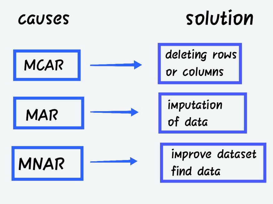
Missing Completely at Random (MCAR)
When the probability of missing data is unrelated to the precise value to be obtained or the collection of observed answers.
-
Missing at Random (MAR)
When the probability of missing responses is decided by the collection of observed responses rather than the exact missing values expected to be reached.
- Missing not at Random (MNAR)
Other than the above-mentioned categories, MNAR is the missing data. The MNAR data cases are a pain to deal with. Modelling the missing data is the only way to get a fair approximation of the parameters in this situation.
Categories of Missing values
Columns with missing values fall into the following categories:
- Continuous variable or feature – Numerical dataset i.e., numbers may be of any kind
- Categorical variable or feature – it may be numerical or objective kind. Ex: customer rating: Poor, Satisfactory,
Good, Better, Best, or Gender: Male or Female.
For either of these two kinds of categories only we will be having our dataset.
Types of Imputations
Imputations are available in a range of sizes and forms. It’s one of the approaches for resolving missing data issues in a dataset before modelling our application for more precision.
- Univariate imputation, or mean imputation, is when values are imputed using only the target variable.
- Multivariate imputation: Impute values depending on other factors, such as estimating missing values based on other variables using linear regression.
- Single imputation: To construct a single imputed dataset, only impute any missing values once inside the dataset.
- Numerous imputations: imputation of the same missing values multiple times inside the dataset. This essentially entails repeating a single imputation to obtain numerous imputed datasets.
How to overcome Missing data in our dataset?
There are many ways to overcome the missing data, we will see methods, before that we will start with the scratch like importing the libraries,
Dataset: https://github.com/JangirSumit/data_science/blob/master/18th%20May%20Assignments/case%20study%201/SalaryGender.csv with modified PhD as categorical
at the beginning of every code, we need to import the libraries,
checking for the dimension of the dataset
dataset.shape
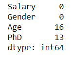
Checking for the missing values
print(dataset.isnull().sum())
-
Just leave it as it is! (Don’t Disturb)
Don’t do anything about the missing data. You hand over total control to the algorithm over how it responds to the data. On the other hand, various algorithms react differently to missing data. Some algorithms, for example, identify the best imputation values for missing data based on training loss reduction. Take XGBoost, for example. In some cases, such as linear regression, an error will occur. It simply means that you’ll have to deal with missing data either during the pre-processing phases or when the model fails, and we’ll have to figure out what went wrong. This section is basically like a trial and error technique; depending on the reaction, we’ll proceed.
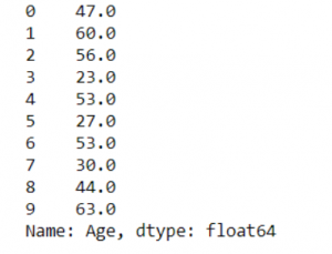
#old dataset with missed values
dataset["Age"][:10]
2. Drop it if it is not in use (mostly Rows)
Excluding observations with missing data is the next most easy approach. However, you run the risk of missing some critical data points as a result. You may do this by using the Python pandas package’s dropna() function to remove all the columns with missing values. Rather than eliminating all missing values from all columns, utilize your domain knowledge or seek the help of a domain expert to selectively remove the rows/columns with missing values that aren’t relevant to the machine learning problem.
Pros: after removing missed data, the model becomes robust
Cons: Loss of data, which may be important too. If you have more missing data then efficiency won’t be good for modelling.
#deleting rows - missed vales
dataset.dropna(inplace=True)
print(dataset.isnull().sum())
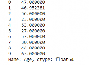
3. Imputation by Mean:
Using this approach, you may compute the mean of a column’s non-missing values, and then replace the missing values in each column separately and independently of the others. The most significant disadvantage is that it can only be used with numerical data. It’s a simple and fast method that works well with small numerical datasets. However, there are certain limitations, such as the fact that feature correlations are ignored. It only works for a single column at a time. Furthermore, if the outlier treatment is skipped, a skewed mean value will almost certainly be substituted, lowering the model’s overall quality.
Cons: Works only with numerical datasets and failed in covariance between the independent variables
#Mean - missed value
dataset["Age"] = dataset["Age"].replace(np.NaN, dataset["Age"].mean())
print(dataset["Age"][:10])
4. Imputation by Median:
Another technique of imputation that addresses the outlier problem in the previous method is to utilize median values. When sorted, it ignores the influence of outliers and updates the middle value that occurred in that column.
Cons: Works only with numerical datasets and failed in covariance between the independent variables
#Median - missed value
dataset["Age"] = dataset["Age"].replace(np.NaN, dataset["Age"].median())
print(dataset["Age"][:10])
5. Imputation by Most frequent values (mode):
This method may be applied to categorical variables with a finite set of values. To impute, you can use the most common value. For example, whether the available alternatives are nominal category values such as True/False or conditions such as normal/abnormal. This is especially true for ordinal categorical factors such as educational attainment. Pre-primary, primary, secondary, high school, graduation, and so on are all examples of educational levels. Unfortunately, because this method ignores feature connections, there is a danger of data bias. If the category values aren’t balanced, you’re more likely to introduce bias into the data (class imbalance problem).
Pros: Works with all formats of data.
Cons: Covariance value cannot be predicted between independent features
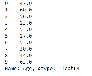
#Mode - missed value
import statistics
dataset["Age"] = dataset["Age"].replace(np.NaN, statistics.mode(dataset["Age"]))
print(dataset["Age"][:10])
6. Imputation for Categorical values:
When categorical columns have missing values, the most prevalent category may be utilized to fill in the gaps. If there are many missing values, a new category can be created to replace them.
Pros: Good for small datasets. Compliments the loss by inserting the new category
Cons: Cant able to use for other than
categorical data, additional encoded features may result in a drop inaccuracy
#missing values - categorical

dataset.isnull().sum()


#missing values - categorical - solution

dataset["PhD"] = dataset["PhD"].fillna('U')


#checking for missed values in Categorical - cabin

dataset.isnull().sum()
7. Last observation carried forward (LOCF)
It is a common statistical approach for the analysis of longitudinal repeated measures data when some follow-up observations are missing.
#LOCF - last observation carried forward

dataset["Age"] = dataset["Age"].fillna(method ='ffill')

dataset.isnull().sum()
8. Interpolation – Linear
It’s the method of approximating a missing value by joining dots in increasing order along a straight line. In a nutshell, it calculates the unknown value in the same ascending order as the values that came before it. Because Linear Interpolation is the default method, we didn’t have to specify it while utilizing it. It will almost always be utilized in a time-series dataset.
#interpolation - linear

dataset["Age"] = dataset["Age"].interpolate(method='linear', limit_direction='forward', axis=0)

dataset.isnull().sum()
9. Imputation by K-NN:
A fundamental classification approach is the k-nearest-neighbors (kNN) algorithm. Class membership is the outcome of k-NN categorization. An item’s categorization is determined by how closely it resembles the points in the training set, with the object going to the class with the most members among its k closest neighbors. If k = 1, the item is simply assigned to the class of the item’s closest neighbor. Finding the k’s closest neighbours to the observation with missing data and then imputing them based on the non-missing values in the neighborhood might help generate predictions about the missing values.
#for knn imputation - we need to remove normalize the data and categorical data we need to convert

cat_variables = dataset[['PhD']]

cat_dummies = pd.get_dummies(cat_variables, drop_first=True)

cat_dummies.head()


dataset = dataset.drop(['PhD'], axis=1)

dataset = pd.concat([dataset, cat_dummies], axis=1)

dataset.head()


#removing unwanted features

dataset = dataset.drop(['Gender'], axis=1)

dataset.head()


#scaling mandatory before knn

from sklearn.preprocessing import MinMaxScaler

scaler = MinMaxScaler()

dataset = pd.DataFrame(scaler.fit_transform(dataset), columns = dataset.columns)

dataset.head()


#knn imputer

from sklearn.impute import KNNImputer

imputer = KNNImputer(n_neighbors=3)

dataset = pd.DataFrame(imputer.fit_transform(dataset),columns = dataset.columns)


#checking for missing

dataset.isnull().sum()
10. Imputation by Multivariate Imputation by Chained Equation (MICE):
MICE is a method for replacing missing data values in data collection via multiple imputations. You can start by making duplicate copies of the data set with missing values in one or more of the variables.
#MICE
import numpy as np
import pandas as pd
from sklearn.experimental import enable_iterative_imputer
from sklearn.impute import IterativeImputer
df = pd.read_csv('https://raw.githubusercontent.com/datasciencedojo/datasets/master/titanic.csv')
df = df.drop(['PassengerId','Name'],axis=1)
df = df[["Survived", "Pclass", "Sex", "SibSp", "Parch", "Fare", "Age"]]
df["Sex"] = [1 if x=="male" else 0 for x in df["Sex"]]
df.isnull().sum()
imputer=IterativeImputer(imputation_order='ascending',max_iter=10,random_state=42,n_nearest_features=5)
imputer
imputed_dataset = imputer.fit_transform(df)
Notes:
For our dataset, we may use the aforementioned ideas to solve for missing values. There is no one approach that is preferable for discovering missing values in this case; the solution for finding missing values varies depending on the missing values in our feature and the application that we will utilize. So, we’ll have to figure it out through trial and error to determine what the optimal option is for our application.
Conclusion:
Did you find this article to be useful? Please leave your thoughts/opinions in the comments area below. Learning from your mistakes is my favourite quote; if you find something incorrect, simply highlight it; I am eager to learn from students like you.
About me in short, I am Premanand.S, Assistant Professor Jr and a researcher in Machine Learning. Love to teach and love to learn new things in Data Science. Mail me for any doubt or mistake, [email protected], and my Linkedin https://www.linkedin.com/in/premsanand/


