A broader understanding of ML and types of regression

Introduction

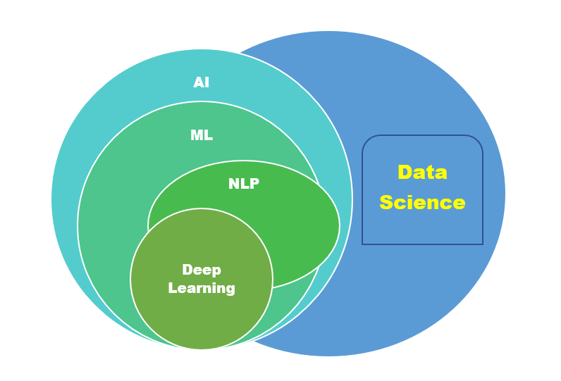
Machine Learning(ML) is the science of interpreting the data and automating the functioning of data analytics by training it through the existing data so that it makes a decision when a similar type of data is passed to it. ML comes under AI(Artificial intelligence) umbrella and many others come under AI where there is a creation of intelligent systems. Below is a small diagram I made for representing AI, ML, and Data Science.

Today, examples of machine learning are all around us. Digital assistants (like Siri, Alexa, Google) work in response to our voice commands. Websites recommend products and movies and songs based on what we bought, watched, or listened to before is how Recommendation systems came up. Robots vacuum our floors while we do other things. I think people can find these robots to buy at e-commerce stores as home assistants. How the technology evolved for our service?

Yes!!! Spam detectors stop unwanted emails is done using NLP. Medical image analysis systems help doctors spot tumors they might have missed with good precision which is helping in detecting our ailments in medical diagnosis. The first self-driving cars are hitting the road in advanced countries and soon will be in our own country also. This is how technology has made our living so easy and hassle-free.

ML Classification:

Machine Learning is classified into four types. They are Supervised, Unsupervised, Semi-supervised, and Reinforcement Learning. Supervised Learning deals with the model being trained with labeled data and making predictions on it. It is easy to evaluate these models as the true values(correct values) are already known. Unsupervised Learning deals with unlabelled datasets where there are no labels given to them or which cannot be given to them.

These models identify the unidentified patterns in it to make predictions. Semi-supervised is the combination of both supervised and unsupervised where some of the data contain labels and others don’t. During training, it uses a smaller labeled data set to guide classification and feature extraction from a larger, unlabeled data set. Reinforcement Learning is like trial and error methods where the correct predictions are rewarded and the incorrect predictions model is penalized and retrained for actions.

ML is mostly used on datasets where Supervised and Unsupervised are the common techniques used for getting the information from it. The other types are also used then firstly the first two classifications are to be known which helps in understanding the latter types well.

Supervised Learning is further classified into two types. They are Regression and Classification tasks. Regression is used for predicting the continuous values and Classification in predicting the discrete values. More clearly, Regression is used for numerical value prediction and Classification for categorical data prediction. Eg: Regression is used for the prediction of house prices, Stock prices, fare prediction, ..etc.Classification is used for the prediction of medical diagnosis(disease is present or not), fraud detection(fraud or no fraud), Rain forecast(Rain or no rain), etc.

There are many models for solving Regression problems like Linear Regression, KNN, SVR, Decision Tree, Random Forest, Boosting methods, and many more.

Predictive Analytics and various other types of analytics:

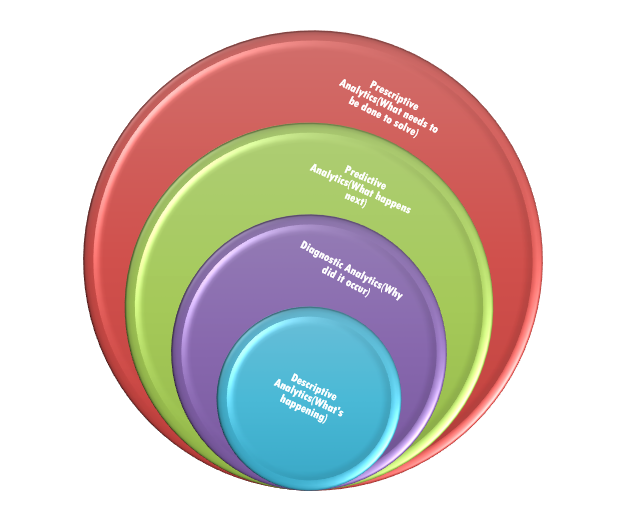
There are four types of analytics. They are Descriptive, Diagnostic, Predictive, and Prescriptive analytics. ML algorithms come under Predicting modeling techniques. Below is the pictorial representation I have made for understanding the types of analytics.

 

Regression analysis to deal with Regression problems in ML and for various other findings in the data:

Regression analysis is used for knowing the relationship between the independent(predictor variables) and dependent(predicted) variables. This technique is used for forecasting, time series modeling, and finding the causal effect relationship between the variables.

Some of the regression techniques used for analysis are Linear Regression, Polynomial Regression, Ridge Regression, Lasso Regression, Elastic net Regression, and Stepwise regression.

1. Linear Regression

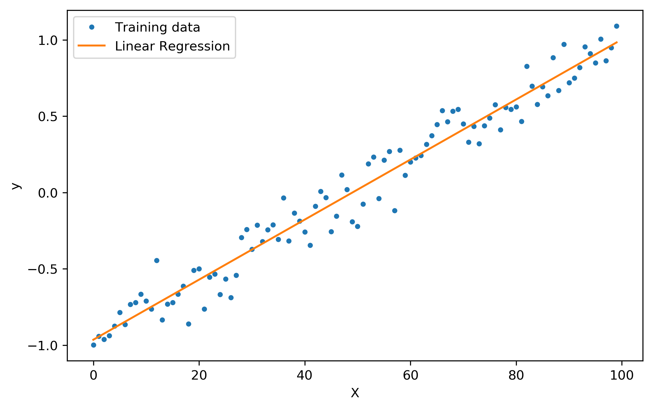
This is also known as OLS(Ordinary least squares)method or Linear least squares method. The linear regression is represented by the equation y= a + bx + e where x = independent variable, a = intercept, b = slope of the line and e = error term. The simple linear regression contains one independent variable whereas multiple linear regression contains more than one independent variable then the equation turns out be y = b0 + b1x1 + b2x2 + …bnxn + e where b0 = intercept; b1,b2,b3..bn = slope of the line, x1,x2,x3…xn = independent variables or features, e = error term.

The assumptions of Linear regression are:

1. Linearity: The relationship between X and Y is linear.
2. Homoscedasticity: The variance of residual is the same for any value of X.
3. Independence: Observations are independent of each other. No correlation between error terms. The absence of this phenomenon is Autocorrelation.
4. No Multicollinearity: There should not be multicollinearity in the regression model. Multicollinearity occurs when there is a high correlation between two independent variables.
5. Normality: For any fixed value of X, Y is normally distributed. The error terms must be normally distributed.

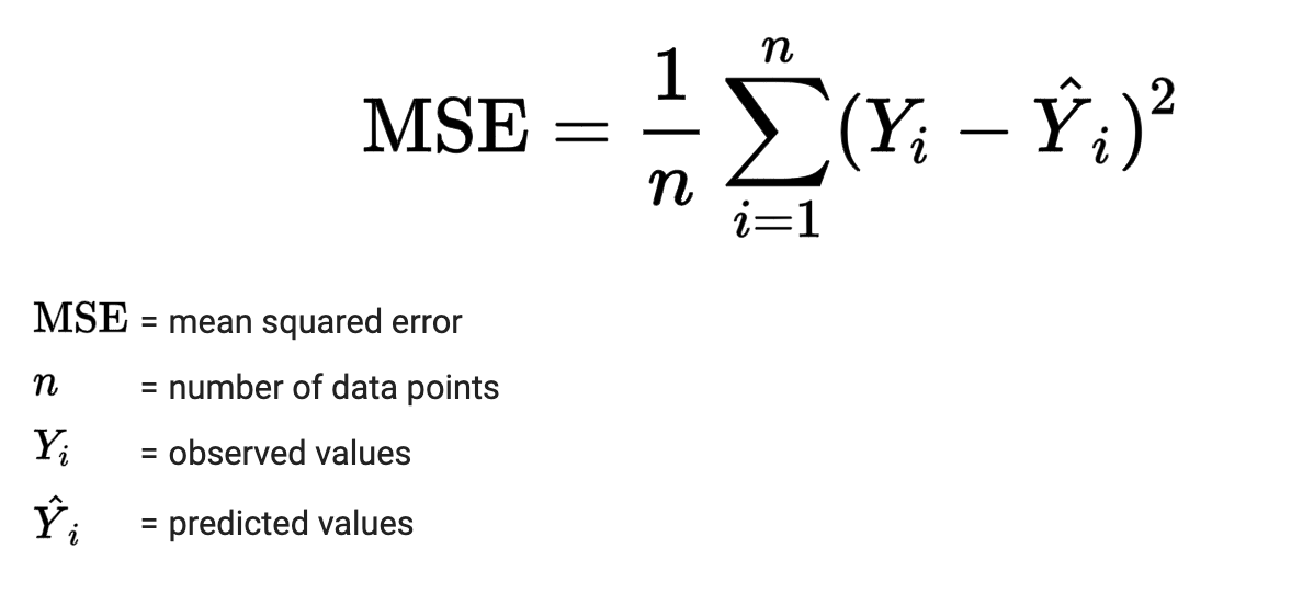
The best fit line is constructed like the above based on all the data points where the loss function is minimum or the error is less that becomes the best fit line for the data. Gradient descent algorithm gives different weights to the equation and using different learning rates whichever gets the minima/maxima cost function becomes the parameters for the linear equation y = a + bx + e. The cost function used to minimize the linear equation error rate is the mean squared error. The equation for it is given below:

When you have got the above stats implementation is just a few code blocks away.

from sklearn.linear_model import LinearRegression
from sklearn.metrics import r2_score
model=LinearRegression()
model.fit(x_train,y_train)
pred=model.predict(x_test)
r2_score(y_test,pred) #for finding r2 score of the predicted and true values

You can explore Linear Regression parameters in the Linear Regression sklearn library

2. Lasso Regression

This is also known as L1 Regression. Lasso is the short form for the Least absolute shrinkage and selection operator. Lasso penalizes the absolute size of the regression coefficients. Regularized linear regression models are very similar to least squares followed in Linear Regression, except that the coefficients are estimated by minimizing a slightly different objective function. We minimize the sum of RSS and a “penalty term” that penalizes coefficient size. The larger the penalty applied, the further the estimates or values get shrunk towards absolute zero. This results in variable selection out of given variables. The equation to find the loss function for L1 is given below:

3. Ridge Regression

This is also known as L2 Regression. Ridge regression acts as a remedial measure used to ease collinearity in between predictors of a model, since, the model includes correlated featured variables, so the final model is confined and rigid in its maximum approach. L2 eliminates the problem of the data facing multicollinearity between the variables.

4. Elastic Net Regression or Regularisation

This is the combination of both L1 and L2 regularization to get the benefits of both methods. Now on using this error decreases a lot compared to using one of it. It uses both Lasso as well as Ridge Regression regularization to remove all unnecessary coefficients but not the informative ones. The below is the equation to calculate it;

 

5. Polynomial Regression

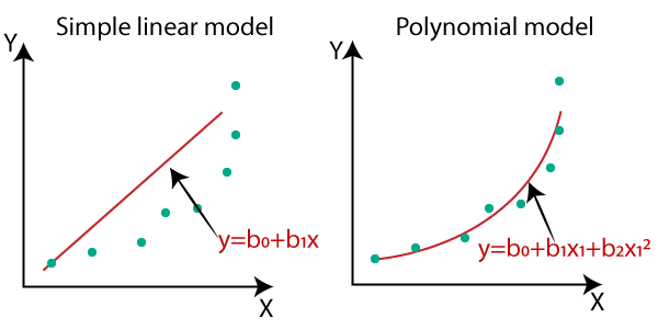
The linear regression works well only with linear data whereas polynomial regression is used for non-linear or when the data points are in the form of a curve. When executing a model that is fit to manage non-linearly separated data, the polynomial regression technique is used. In it, the best-fitted line is not straight, instead, a curve that best-fitted to data points.

The equation for polynomial equation comes in the form of degrees based on the variables available or the number of features to be fit in polynomial regression. The equation for it is y = b0 + b1x1 + b2x2^2 + b3x3^3 +……+ bnxn^n, where b0 = intercept, b1,b2,b3..bn = intercept of the polynomial regression curve, x1,x2^2…..xn^n = the n square of xn variables represent the independent variables squared up to the degree of the polynomial.

 

6. Stepwise Regression

In this method, regression is constructed until and unless all the variables are in the required p-value or t-stats or test statistic. With every forward step, the variable gets added or subtracted from a group of descriptive variables.

The criteria followed in the stepwise regression technique are forward determination (forward selection), backward exclusion (backward elimination), and bidirectional removal (bidirectional elimination). This is achieved by observing statistical values like R-square, t-stats, and AIC metric to discern significant variables. Stepwise regression fits the regression model by adding/dropping co-variates one at a time based on a specified criterion.

There are many ways to do feature selection instead of Univariate Feature selection using stats(p-value,f test, chi-square).UFS selects features based on univariate statistical tests, which evaluate the relationship between two randomly selected variables. In the case of a continuous dependent variable, two options are available: f-regression and mutual_info_regression.

Several options are available but two different ways of specifying the removal of features are (a) SelectKBest removes all low scoring features, and (b) SelectPercentile allows the analyst to specify a scoring percent of features, and all features not reaching that threshold then are removed. To do this different methods like OLS, RFE(Recursive feature elimination), RFECV(Recursive feature elimination and cross-validation), SelectKBest, GenericUnivariateSelect. Feature selection using SelectFromModel allows the analyst to make use of L1-based feature selection (e.g. Lasso) and tree-based feature selection. All the above methods are available in sklearn.

This is a summary made for understanding Machine Learning and some of the statistics linked with Regression models. Let me know if there are any questions and difficulties in it or any other related queries. Thanks for reading.😎 Have a nice day.😊

YAMINI PEDDIREDDI

24 Apr 2021