A Brief Introduction to Linear Discriminant Analysis

This article was published as a part of the Data Science Blogathon

Introduction to LDA:

Linear Discriminant Analysis as its name suggests is a linear model for classification and dimensionality reduction.  Most commonly used for feature extraction in pattern classification problems. This has been here for quite a long time. First, in 1936 Fisher formulated linear discriminant for two classes, and later on, in 1948 C.R Rao generalized it for multiple classes. LDA projects data from a D dimensional feature space down to a D’ (D>D’) dimensional space in a way to maximize the variability between the classes and reducing the variability within the classes.

Why LDA?:

• Logistic Regression is one of the most popular linear classification models that perform well for binary classification but falls short in the case of multiple classification problems with well-separated classes. While LDA handles these quite efficiently.
• LDA can also be used in data preprocessing to reduce the number of features just as PCA which reduces the computing cost significantly.
• LDA is also used in face detection algorithms. In Fisherfaces LDA is used to extract useful data from different faces. Coupled with eigenfaces it produces effective results.

Shortcomings:

• Linear decision boundaries may not effectively separate non-linearly separable classes. More flexible boundaries are desired.
• In cases where the number of observations exceeds the number of features, LDA might not perform as desired. This is called Small Sample Size (SSS) problem. Regularization is required.

We will discuss this later.

Assumptions:

LDA makes some assumptions about the data:

• Assumes the data to be distributed normally or Gaussian distribution of data points i.e. each feature must make a bell-shaped curve when plotted. 
• Each of the classes has identical covariance matrices.

However, it is worth mentioning that LDA performs quite well even if the assumptions are violated.

Fisher’s Linear Discriminant:

LDA is a generalized form of FLD. Fisher in his paper used a discriminant function to classify between two plant species Iris Setosa and Iris Versicolor.

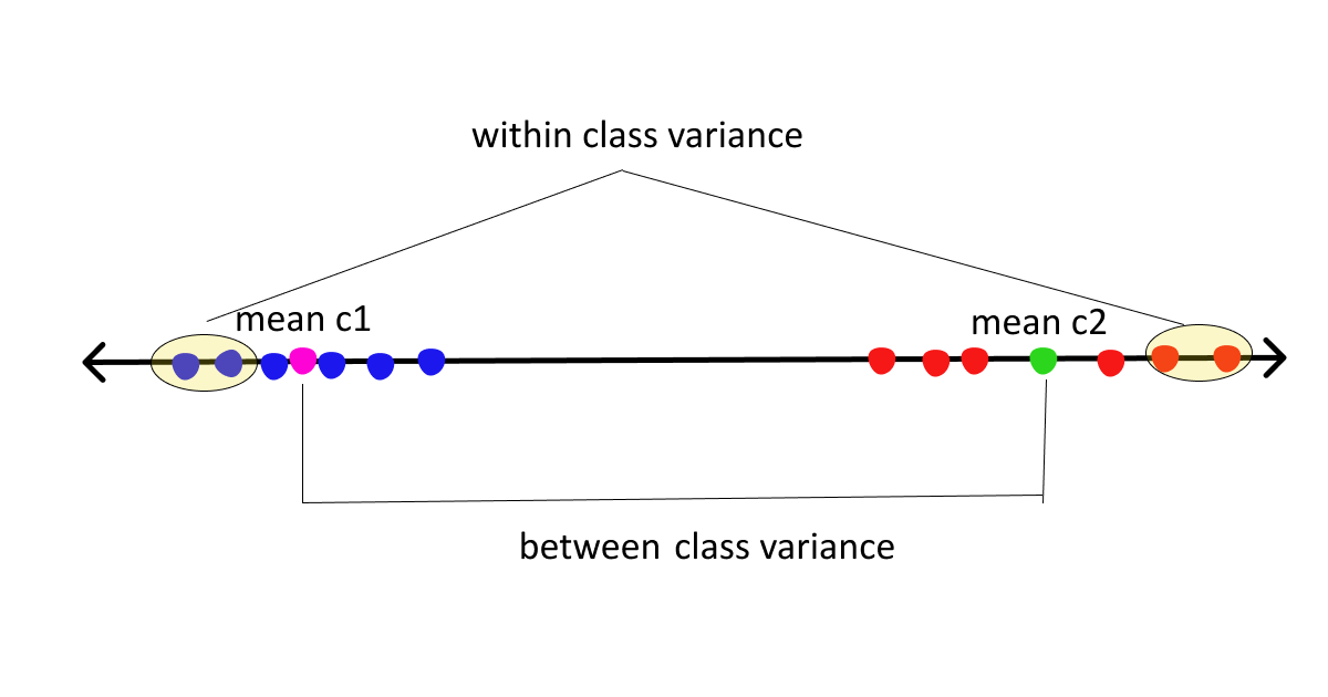
The basic idea of FLD is to project data points onto a line to maximize the between-class scatter and minimize the within-class scatter.

This might sound a bit cryptic but it is quite straightforward. So, before delving deep into the derivation part we need to get familiarized with certain terms and expressions.

• Let’s suppose we have d-dimensional data points x₁….x_n with 2 classes C_i=1,2 each having N₁ & N₂ samples.
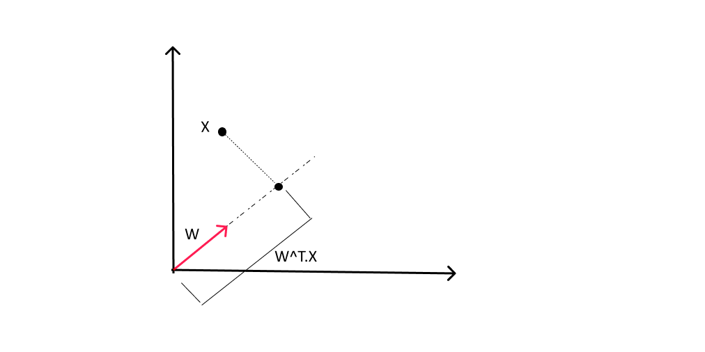
• Let W be a unit vector onto which the data points are to be projected (took unit vector as we are only concerned with the direction).
• Number of samples : N = N1 + N2
• If x(n) are the samples on the feature space then WTx(n) denotes the data points after projection.
• Means of classes before projection: m_i
• Means of classes after projection:  M_i = W^Tm_i

Scatter matrix: Used to make estimates of the covariance matrix. IT is a m X m positive semi-definite matrix.

Given by: sample variance * no. of samples.

Note: Scatter and variance measure the same thing but on different scales. So, we might use both words interchangeably. So, do not get confused.

Here we will be dealing with two types of scatter matrices

• Between class scatter = S_b = measures the distance between class means
• Within class scatter = Sw = measures the spread around means of each class

Now, assuming we are clear with the basics let’s move on to the derivation part.

As per Fisher’s LDA :

arg max J(W) = (M₁ – M₂)² / S₁² + S₂²       ………..    (1)

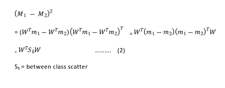
The numerator here is between class scatter while the denominator is within-class scatter. So to maximize the function we need to maximize the numerator and minimize the denominator, simple math. To maximize the above function we need to first express the above equation in terms of W. 

Numerator:

Denominator:

For denominator we have S₁² + S₂²  . 

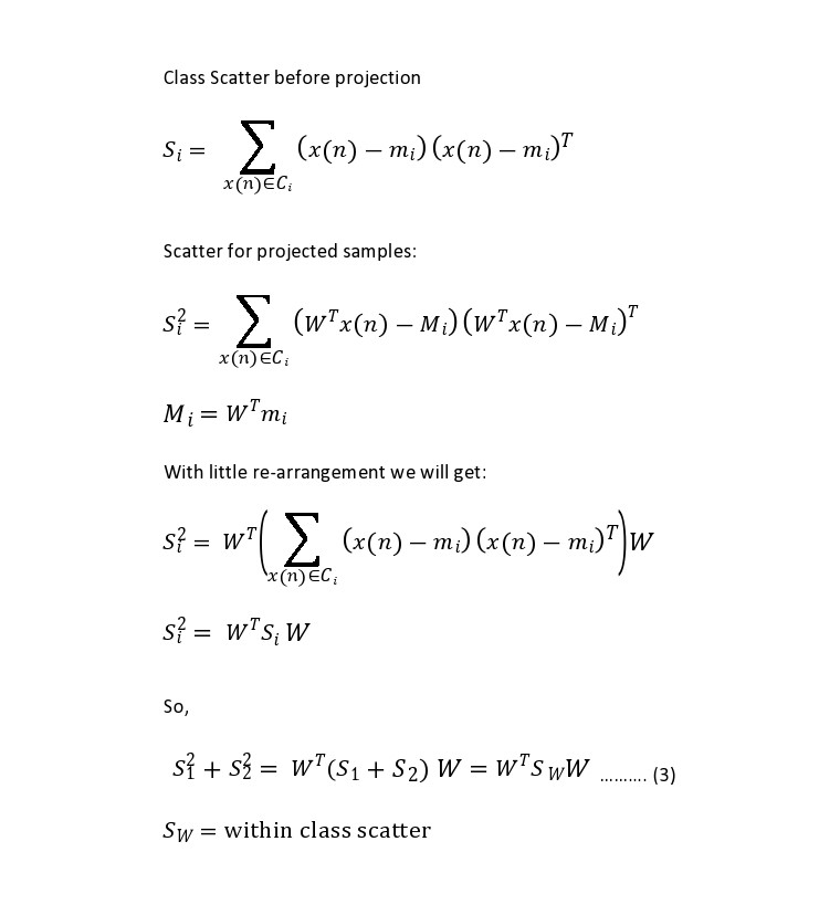
Now, we have both the numerator and denominator expressed in terms of W

J(W) = W^TS_bW / W^TS_wW

Upon differentiating the above function w.r.t W and equating with 0, we get a generalized eigenvalue-eigenvector problem

S_bW = vS_wW    

S_w being a full-rank matrix , inverse is feasible

=> S_w^-1S_bW = vW

_{Where v = eigen value}

_{W = eigen vector}

LDA for multiple classes:

LDA can be generalized for multiple classes. Here are the generalized forms of between-class and within-class matrices.

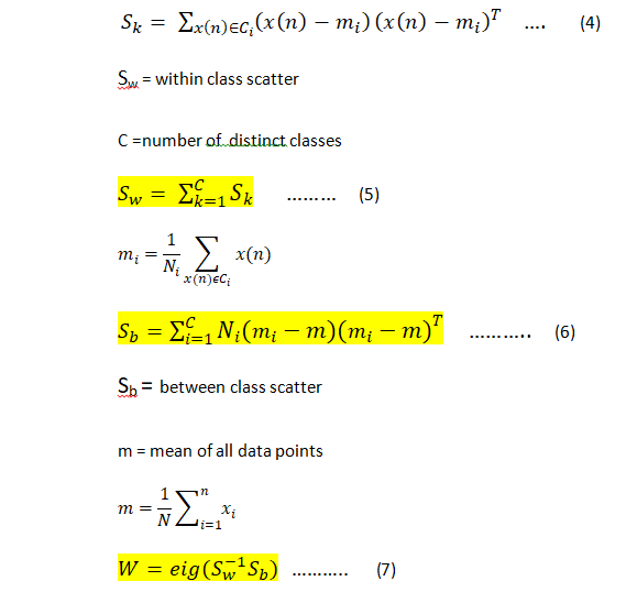
Note: S_b is the sum of C different rank 1 matrices. So, the rank of S_b <=C-1. That means we can only have C-1 eigenvectors. Thus, we can project data points to a subspace of dimensions at most  C-1.

Above equation (4) gives us scatter for each of our classes and equation (5) adds all of them to give within-class scatter. Similarly, equation (6) gives us between-class scatter. Finally, eigendecomposition of S_w^-1S_b gives us the desired eigenvectors from the corresponding eigenvalues. Total eigenvalues can be at most C-1.

LDA for classification:

Until now, we only reduced the dimension of the data points, but this is strictly not yet discriminant. But the projected data can subsequently be used to construct a discriminant by using Bayes’ theorem as follows.

Assume X = (x₁….x_p) is drawn from a multivariate Gaussian distribution. K be the no. of classes and Y is the response variable. pik is the prior probability: the probability that a given observation is associated with K^th class. Pr(X = x | Y = k) is the posterior probability.

Let f_k(X) = Pr(X = x | Y = k) is our probability density function of X for an observation x that belongs to K^th class. f_k(X) is large if there is a high probability of an observation in  K^th class has X=x. 

As per Bayes’ theorem,

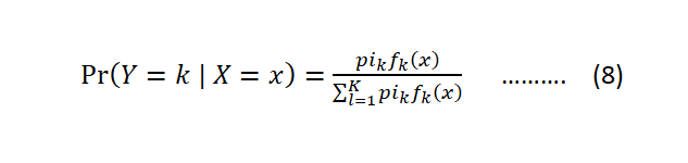
Now, to calculate the posterior probability we will need to find the prior pi_k and density function f_k(X). 

pik can be calculated easily. If we have a random sample of Ys from the population: we simply compute the fraction of the training observations that belong to Kth class. But the calculation of f_k(X) can be a little tricky.

We assume that the probability density function of x is multivariate Gaussian with class means m_k and a common covariance matrix sigma.

As a formula, multi-variate Gaussian density is given by:

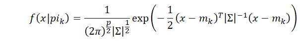
|sigma| = determinant of covariance matrix ( same for all classes)

m_k = class means

Now, by plugging the density function in the equation (8), taking the logarithm and doing some algebra, we will find the Linear score function

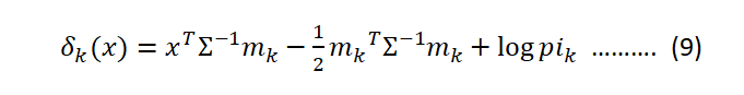
We will classify a sample unit to the class that has the highest Linear Score function for it.

Note that in the above equation (9) Linear discriminant function depends on x linearly, hence the name Linear Discriminant Analysis.

Addressing LDA shortcomings

Linearity problem: LDA is used to find a linear transformation that classifies different classes. But if the classes are non-linearly separable, It can not find a lower-dimensional space to project. This problem arises when classes have the same means i.e, the discriminatory information does not exist in mean but in the scatter of data. That will effectively make S_b=0. To address this issue we can use Kernel functions. As used in SVM, SVR etc. The idea is to map the input data to a new high dimensional feature space by a non-linear mapping where inner products in the feature space can be computed by kernel functions.

Small Sample problem: This problem arises when the dimension of samples is higher than the number of samples (D>N). This is the most common problem with LDA. The covariance matrix becomes singular, hence no inverse. So, to address this problem regularization was introduced. Instead of using sigma or the covariance matrix directly, we use

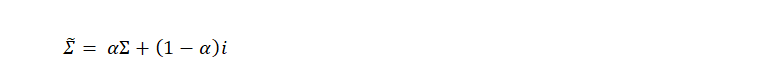
Here, alpha is a value between 0 and 1.and is a tuning parameter. i is the identity matrix. The diagonal elements of the covariance matrix are biased by adding this small element. However, the regularization parameter needs to be tuned to perform better.

Scikit Learn’s LinearDiscriminantAnalysis has a shrinkage parameter that is used to address this undersampling problem. It helps to improve the generalization performance of the classifier. when this is set to ‘auto’, this automatically determines the optimal shrinkage parameter. Remember that it only works when the solver parameter is set to ‘lsqr’ or ‘eigen’. This can manually be set between 0 and 1.There are several other methods also used to address this problem. Such as a combination of PCA and LDA. PCA first reduces the dimension to a suitable number then LDA is performed as usual.

Python Implementation:

Fortunately, we don’t have to code all these things from scratch, Python has all the necessary requirements for LDA implementations. For the following article, we will use the famous wine dataset.

Python Code:

Fitting LDA to wine dataset:

lda = LinearDiscriminantAnalysis()
lda_t = lda.fit_transform(X,y)

Variance explained by each component:

lda.explained_variance_ratio_

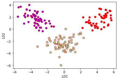
Plotting LDA components:

plt.xlabel('LD1')
plt.ylabel('LD2')
plt.scatter(lda_t[:,0],lda_t[:,1],c=y,cmap='rainbow',edgecolors='r')

LDA for classification:

X_train,X_test,y_train,y_test = train_test_split(X,y,test_size=0.3)
lda.fit(X_train,y_train)

Accuracy Score:

y_pred = lda.predict(X_test)
print(accuracy_score(y_test,y_pred))

Confusion Matrix:

confusion_matrix(y_test,y_pred)

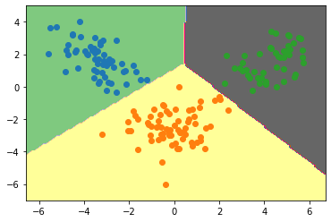
Plotting Decision boundary for our dataset:

min1,max1 = lda_t[:,0].min()-1, lda_t[:,0].max()+1
min2,max2 = lda_t[:,1].min()-1,lda_t[:,1].max()+1
x1grid = np.arange(min1,max1,0.1)
x2grid = np.arange(min2,max2,0.1)
xx,yy = np.meshgrid(x1grid,x2grid)
r1,r2 = xx.flatten(),yy.flatten()
r1,r2 = r1.reshape((len(r1),1)), r2.reshape((len(r2),1))
grid = np.hstack((r1,r2))

model = LinearDiscriminantAnalysis()
model.fit(lda_t,y)
yhat = model.predict(grid)
zz = yhat.reshape(xx.shape)
plt.contourf(xx,yy,zz,cmap='Accent')

for class_value in range(3):
  row_ix = np.where( y== class_value)
  plt.scatter(lda_t[row_ix,0],lda_t[row_ix,1])

Conclusion

Linear Discriminant Analysis (LDA) stands out as a valuable tool for simplifying data and making classifications. We’ve covered why LDA is important, its limitations, and key components such as Fisher’s Linear Discriminant. Understanding the numerator and denominator in LDA, its application for multiple classes, and its implementation in Python provides practical insights. Recognizing and addressing LDA’s limitations is crucial for effective use in diverse scenarios.

So, this was all about LDA, its mathematics, and its implementation. Hope it was helpful.

Thanks for reading.

FAQs

Source: An Introduction to Statistical Learning with Applications in R – Gareth James, Daniela

Sunil Kumar Dash

20 Nov 2023